Notes: More Sampling Methods

Containing an incomplete overview of additional methods for generating samples from a posterior PDF.

Optional extra reading material

• Handbook of MCMC (Brooks, Gelman, Jones and Meng, eds.), parts of which are on the web
• Recent and less recent notes on CosmoMC by Antony Lewis
• Method-specific links below

Overview

The Metropolis-Hastings algorithm has historically been the workhorse MCMC method, in that it is widely applicable, its inner workings and shortcomings are relatively simple to understand, and it's straightforward to assess how well it's working. But that doesn't mean it's the only or best solution for any particular problem.

I would caution against thinking of the methods below as more "advanced", in the sense of being automatically preferable, compared with those we have already seen. For example, several of them are "better" in the sense that the sequences they produce tend to be less correlated than Metropolis would yield. Yet, we've seen that correlated chains are not a bug, as such. In practice, what we care about is accumulating a certain number of effectively independent samples in a reasonable amount of human time, with the run time determined by the number of times the posterior needs to be evaluated. An algorithm that produces completely independent samples, but requires 10 posterior evaluations for each one, is no better according to this metric than a Metropolis kernel with a correlation length of 10.

All of which is to say that, in my limited experience, this is one of those cases where there just isn't a free lunch to be had. Compared to Metropolis with the most straightforward and common-sense proposal adaptation (see below), other methods that I've tried (which, admittedly, does not include everything below) haven't been any faster. Since many of those methods don't admit the same simple diagnostics that we saw previously, I tend to stubbornly stick with Metropolis (or conjugate Gibbs, when possible) in my own work. But that doesn't mean you shouldn't learn about and try other things. And there are certain tasks that MCMC methods simply don't do well, like calculation of the Bayesian evidence, for which we'll want to use other approaches (see Model Evaluation and Comparison II).

One thing to keep in mind, when faced with a very computationally expensive problem, is that we're allowed to use different samplers for different subsets of parameters, just as long as every parameter gets updated somehow.

Accelerating Metropolis

Our first method is not actually a novel one, just our old friend Metropolis with extra bells and whistles. Recall the basic algorithm:

choose a starting point and a proposal scale
while we want more samples
    propose a new point from a scaled distribution, centered on our current position
    accept/reject the new point

To speed things up in human time, we can also take advantage of the embarrassingly parallel nature of the algorithm. That is, nothing prevents us from running multiple, independent chains using as many CPUs as we have available, and pooling the chains at the end. In fact, we've seen that we'll want multiple chains in any case, to test for convergence.

In the algorithm itself, we mainly have freedom to play with the proposal distribution. We've already discussed using a proposal distribution that discourages very small steps (in scaled units). What else can we do? The better we can tune the proposal distribution to match the overall shape of the posterior, the more efficiently the chain will be able to move around in parameter space. Hence, the goal is to cleverly and automatically tune the proposal distribution.

Strictly speaking, tuning the proposal distribution on the fly breaks the rules of MCMC (specifically, detailed balance). Technically, we should stop tuning after some time, once things appear to be working well, and throw away all steps before that point. In practice, if we've actually managed to converge to the target distribution, subsequent updates to the proposal distribution will be negligible anyway, making this less of a concern.

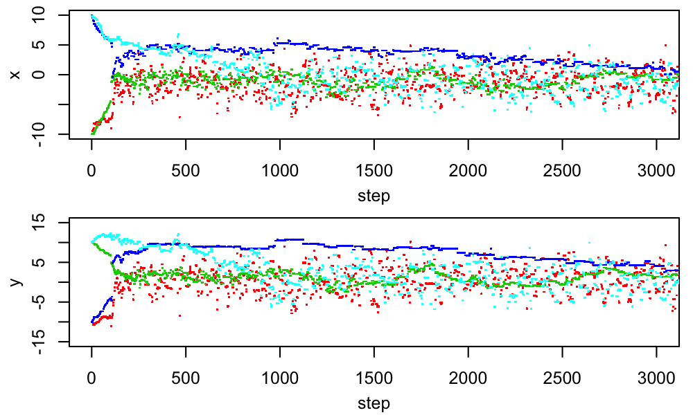
Adapting the proposal distribution

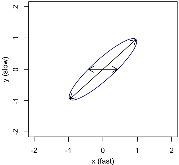
One way of making the proposal distribution more efficient would be to customize the proposal scale for each parameter. If we believe the chain has begun (laboriously) to sample from the posterior, we could periodically compute the standard deviation of the samples so far in each direction, and use that as a guess of the appropriate proposal scale. More generally, we could look at the multidimensional covariance of the samples so far, and adjust the shape of our proposal distribution to match; this would let us learn about and compensate for parameter degeneracies. This change is equivalent to using a rotated coordinate basis, with appropriate scales in each new basis direction, for our proposal distribution. We could visualize it like this:

Original

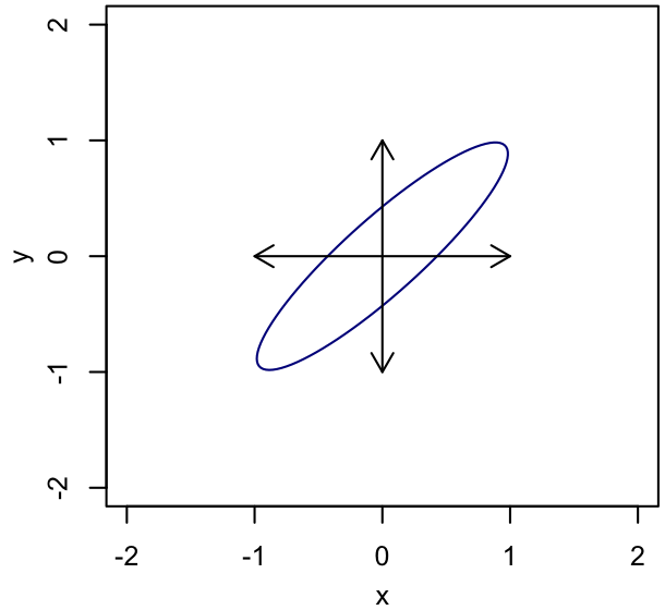
Proposal basis change

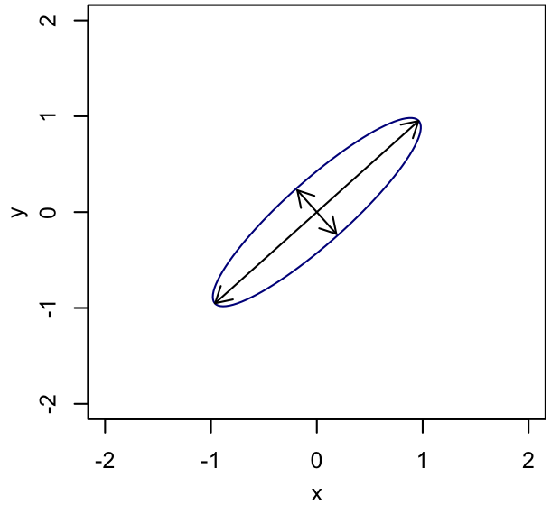
Parameter basis change

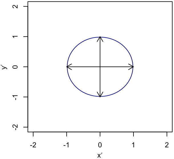
In each panel, the ellipse shows the shape of the posterior distribution, and the vectors show the coordinate basis with respect to which the proposal distribution is defined. (We are not confined to proposing along these directions, but are imagining that we want the proposal distribution to be simple with respect to this basis, and have a proposal scale associated with each basis direction.) On the left, the basis is Cartesian, with the scales set to the standard deviation of the (marginal) posterior in each direction; we can see that this results in proposals that are too large on average to be accepted often. In the center, we have rotated the basis for proposals to align with the major and minor axes of the iso-probability surfaces, and tuned the associated scales appropriately. This can equivalently be accomplished by re-defining the parameters to reduce the correlation of the PDF, as illustrated on the right. (Note that, being a rotation and scaling, this parameter transformation is linear, meaning that the priors are invariant under it. If we had used a nonlinear reparametrization, we'd need to worry about transforming the prior density accordingly.) For a nice, elliptical PDF like the one shown, a basis that diagonalizes the covariance matrix is optimal.

Fast-slow decompositions

If changes to some parameters require much more costly calculations than others, straightforward diagonalization of the covariance may not be optimal in practice. In this case, we might want to propose changes to fast parameters more often than slow parameters. More generally, given a hierarchy of speeds, we can also triangularize the proposal basis, such that the fastest parameter appears in every basis vector, the second-fastest appears in all but one, etc., with the slowest parameter being changed only in tandem with all other parameters. This is illustrated in the right panel, below. We might also consider sampling in faster directions more often than in slower directions.

Original

Diagonalized covariance

Triangular fast-slow

Communicating parallel chains

We've already discussed running independent chains in parallel, and using information gathered so far in a chain to adapt the proposal distribution. Combining these ideas turns out to be extremely powerful. If we start multiple chains in different parts of parameter space as usual, and their proposal distributions are not great out of the box, then chances are they will make their way to different parts of the region where the posterior is non-tiny and then struggle to move around. Pooling the information about where multiple chains are sampling can thus tell us much more about the global shape of the posterior than looking only at one chain. With some imagination, we can see this in the example below, where the most degenerate direction becomes evident within the first few steps of each chain.

Pooling information in this way can vastly decrease the time to convergence compared with running separate chains, much more so than the speedup from embarrassingly simple parallelization alone. Consider the comparison of independent-adaptive and communicating-adaptive chains below, where the starting positions and adaptation strategy (diagonalizing the covariance) are the same in each case.

It isn't so easy to tell what's happening as a function of time for each chain in these plots, but, looking at their traces, we see that the communicating chains provide more useful information more quickly than the alternative.

Independent adaptation

Pooled adaptation

As with doing on-the-fly adaptation to begin with, we are breaking a rule here - the chains are no longer independent, so we should think about the consequences for our ability to test for convergence by comparing them. Strictly speaking, we should use a procedure like this strictly to find a good proposal distribution, then throw away those chains and run new ones with the proposal distribution fixed. On the other hand, the argument that the proposal distribution will eventually stop changing still holds (normally), so comparisons of the post-convergence chains are still arguably reasonable. In addition, we still have the sanity check that chains with dispersed starting points found their way to the same part of parameter space, regardless of the adaptation method.

Packages for accelerated Metropolis

Most packaged implementations of Metropolis-Hastings will do at least some of the above; see links in the Monte Carlo Sampling notes.

Parallel tempering

Consider the function $[p(x)]^{1/T}$, where $p(x)$ is the target PDF. We say a chain sampling this function, instead of $p(x)$ itself, has temperature $T$. For $T>1$, $p^{1/T}$ is smoothed out compared with $p$. This smoothed out distribution will be easier to move around than the original, especially when there are strong/complex degeneracies, and in particular it should be more likely for a chain to move between well separated peaks of the PDF. Of course, we're only actually interested in samples obtained for $T=1$, ultimately.

With parallel tempering, we run one chain with $T=1$ and several more chains with $T>1$. A modified Metropolis-Hastings update occasionally allows the chains to exchange positions, giving the $T=1$ chain a mechanism for sampling regions of parameter space it might otherwise have low probability of proposing. Samples from the $T=1$ chain can be used for inference.

Hamiltonian Monte Carlo (HMC) aka Hybrid Monte Carlo (HMC)

While standard MCMC is analogous to the evolution of a thermodynamic system, HMC is (almost) analogous to the dynamical evolution of a single particle. Consider our free parameters as coordinates of a position, $\theta$, and minus the log-posterior as a potential energy, $U(\theta)$.

HMC introduces momentum parameters, $\phi$, corresponding to each position parameter, and an associated "kinetic energy",

$K(\phi) = \sum_i \frac{\phi_i^2}{2m_i}$,

where we are free to choose the "masses", $m_i$. Looking at the analogy the other way, the probability associated with $K(\phi)$,

$p(\phi) \propto e^{-K(\phi)}$,

is a multivariate Gaussian with mean zero and a diagonal covariance given by the masses.

The HMC algorithm alternates direct sampling of $\phi$ from this Gaussian with joint updates of $\phi$ and $\theta$, as follows:

1. Generate a sample of $\phi$ from the distribution defined by $K(\phi)$.
2. Evolve $(\theta,\phi)$ for some time as a dynamical system, according to $K(\phi)$ and $U(\theta)$.
3. The state at the end of this process is the proposal. Apply the standard Metropolis acceptance test to the initial and proposed probabilities $e^{-(K+U)}$. (This is trivial if we conserve energy perfectly in the "evolution" phase, but in practice the evolution is often done more approximately to save time.)

There's a lot more literature on HMC and its optimization than we can cover - see e.g. this chapter. In a nutshell, the introduction of "momentum" into the evolution of the chain is supposed to reduce the random-walk behavior (autocorrelation) of traditional MCMC.

The catch is that, to evolve the $(\theta,\phi)$ state, we need to compute the gradient of the log-posterior (the "force"). If this can be computed analytically, we're in business. If we need to do it numerically, it isn't obvious that HMC will have any advantage over standard MCMC.

These days, there are HMC packages that can perform symbolic differentiation, provided you can express your model as equations in their own language. For complex models, doing this translation such that the resulting, automatically generated code is efficient can be something of an art. And sadly, those of us using complex, legacy likelihood codes that we'd rather not reinvent, or that involve fundamentally non-analytic components like ugly look-up tables, are not likely to move to HMC any time soon.

Some packages for HMC

• PyMC (this is its primary/default method)
• Stan is an independent code that has a Python interface (PyStan).

Intelligent conjugate Gibbs

This is not really a new method, but it's worth knowing that there is software out there that can handle the exploitation of conjugacies for you. Similarly to HMC, you would need to code up your model symbolically; the software then determines what conjugacies exist and uses them, meaning that you don't need to implement those updates yourself (possibly introducing errors). For parameters that are not conjugate, they typically fall back on basic one-parameter-at-a-time Metropolis sampling, so it's only worth investigating these packages if you know (or suspect) your problem has conjugacies to take advantage of.

Packages for Gibbs sampling

See links in the Monte Carlo Sampling notes.

Goodman-Weare sampling

Moving beyond Markov chain methods, the method of Goodman and Weare (2010) works by evolving an ensemble of points in parameter space. After convergence, the ensemble can be regarded as a set of samples from the target distribution. This approach provides some of the benefits of running multiple chains, although we cannot interpret the evolution of the points in the ensemble as independent chains in any sense.

The procedure for moving each point (aka walker) in the ensemble is:

1. Randomly pick a different point from the ensemble (total size $N$).
2. Propose a move in the direction of that point, by the distance between them multiplied by a random number from this distribution:

$g(z) \propto \frac{1}{\sqrt z}; ~ \frac{1}{2}\leq z \leq 2$. 3. Accept or reject the move based on the ratio of posterior densities multiplied by $z^{N-1}$.

Note that there is some magic in the density $g$. We are not free to choose just any function.

This algorithm is relatively easy to use - there is no tuning required and it's straightforward to parallelize. One just needs to provide an initial ensemble, which is not much more onerous than providing a single initial state for MCMC. For these reasons, we lean on a Python implementation called emcee (feel free to groan) in some of the later tutorials. There are some important cautions to keep in mind, however.

• This method can be extremely slow to finding the region where the posterior is large if it is not started there to begin with. Seriously. At least once a year, I get a question like "Everything looked good and converged, until all of a sudden the distribution of walkers blew up and they went everywhere. What's broken?" Nothing's broken. That potentially long early run that looks "perfect" is just walkers swapping with one another because they can't find a better move, perpetuating the original distribution of the ensemble. Eventually they figure it out, at which point they will disperse throughout the (possibly much wider) posterior.
• As the walkers are not independent in any sense, our usual methods for assessing convergence cannot necessarily be trusted (see the story above). Running two independent fits with ensembles started in different places is one possible solution, but that runs into the issue of possibly slow convergence when not starting near the peak probability. Starting with a very spread out ensemble is kind of like chains with different starting positions, but again might be very slow to converge.

In short, we'll use this method when we're already pretty sure that the the posterior is simple (unimodal), that we can guess a decent starting point, and that we'll therefore be able to recognize convergence unambiguously.

Some packages for G-W sampling

• emcee is probably the easiest to jump in and use.
• LMC might be useful if parallelization over MPI is advantageous.

Population Monte Carlo (PMC)

Now we get to some fundamentally different approaches. Recall the essence of MC integration,

$\int f(x) \, dx = \int w(x) \, p(x) \, dx \approx \frac{1}{n}\sum_i w(x_i)$; $x_i \sim p$.

We used this (way back) to motivate Simple Monte Carlo, where $p$ is the prior and $w$ is the likelihood. The key feature that enabled SMC is that any set of points can provide an unbiased estimate of an integral, as long as the weighting is correct.

PMC is a more refined version of this - instead of sampling from the prior, we iteratively build up an approximation to the posterior distribution, called the generating distribution, along with a number of samples and associated weights. Each iteration consists of

1. selecting the generating distribution, $q$,
2. sampling a number of points from the generating distribution, and
3. computing the corresponding posterior densities, $\pi$.

These points can then be weighted by the ratio $\pi/q$ and treated as samples of the posterior. All of these points, that is; no matter which iteration they came from and how uninformed the generating distribution was at that point, they still come with the correct weight. Still, getting accuracy from this method on human timescales requires a clever way to refine $q$. With a suitably intelligent implementation (e.g. see this), the generating distribution can be evolved towards the posterior distribution, providing samples for a posteriori analysis as well as an estimate for the evidence.

Nested sampling

This is a particular form of PMC that is primarily aimed at calculating the Bayesian evidence. We'll look at its utility more closely in the notes on model comparison. In brief, we begin with a large number of points sampled from the prior, and gradually evolve them towards higher-likelihood positions, keeping track of how the volume filled changes (marvel at the complicated math here). Like PMC generally, every time we evaluate the likelihood we get a sample and a weight that we can use to derive parameter constraints, regardless of whether we even care about the evidence.

By virtue of spamming the parameter space with points at the start, nested sampling is likely (though never guaranteed) to find multiple modes, if they exist. The same can be said of PMC, given a wide initial generating distribution. Since these methods maintain something like a global view of the parameter space, rather building up information by tracing a sequence through the space, they are probably the best option in the situation that confounds MCMC, when there are widely separated peaks in the posterior distribution.

If nested sampling is so much more foolproof than MCMC, why wouldn't we always use it instead? In short, exactly those features that make it more robust to multimodal distributions make it less efficient than MCMC for unimodal distributions - if our goal is simply to find the peak and the usual credible intervals/regions, we're better off looking around the region of parameter space where the posterior is large, rather than carefully mapping out the tails.

Some packages for nested sampling

• dynesty, which we will use in a future tutorial.
• UltraNest seems extremely similar, at first glance.

Parting thoughts and general advice

Understanding the guts of every possible sampling algorithm is not really the point of this course, so the list above is necessarily incomplete and somewhat superficial. Hopefully, you've gotten at least a sense of what's out there and how it works.

Like many things in computing, finding the best way to sample a particular PDF when optimization really matters is an art. I'll just reiterate two pieces of advice from above

1. Within a Markov chain setting, it is entirely legitimate to use different algorithms to update different parameters or groups of parameters. Sometimes this might allow you to take advantage of efficiencies that only apply to a subset of parameters. It is also entirely legitimate to directly integrate over a subset of parameters within the posterior calculation rather than sampling them, provided we don't care about having samples of them later on. Again, this might be the most efficient way of dealing with some parameters in a given problem (and it's a strategy we'll use in some of the Practice tutorials).
2. There is no free lunch. Sorry, but it's true. I look forward to being wrong some day, but so far I have yet to see a general algorithm perform significantly better than adaptive Metropolis (with the exception of non-general tricks like conjugacy that take advantage of human intelligence). Fancier samplers might produce prettier (less correlated) samples, but in terms of the number of posterior evaluations needed to get results in the end it seems to be a wash. That said, there certainly could be particular problems where one algorithm really does perform better than others; nested sampling may be the best choice when the posterior is multimodal, for example.

As you've seen already, sampling packages tend to come in two flavors: those with a relatively "minimalist" interface that leaves the user responsible for the model implementation (e.g. emcee, where the user provides initial parameter values and a log-posterior function that accepts a parameter array as an argument), and those where the user is expected to specify the entire model in the package's bespoke pseudocode. There's a trade-off here, in that the latter potentially helps one avoid any number of coding mistakes, but can also make the process of debugging more opaque and/or preclude the use of external codes within the posterior calculation. If you're comfortable with all that, then PyMC is probably a good choice for most purposes, since it's actively developed and has a large user base. Otherwise (and we're open to feedback on this), our advice is emcee to get something up and running quickly in Python, falling back to the Metropolis variant of your choice if there are any doubts about the G-W sampling working correctly, and specialized codes like nested/Gibbs sampling where appropriate.