Notes: Evaluating and Comparing Models (Again!)

In which we will

• Look at tests of model adequacy (goodness of fit), and methods of comparing model fitness
• Understand the use of Bayesian Evidence in this context

So far we have focused on the business of building a probabilistic model and using data to infer the posterior distribution of its parameters. However, model building inevitably requires making assumptions of some kind. No inference problem is really complete until we have assessed whether the data are consistent with those assumptions.

Three related but distinct questions thus come under the heading of model evaluation.

1. Does a model explain (fit) the data well?
2. Does a model make accurate predictions about new data?
3. How probable are our competing models in light of the data?

Often (2) and (3) are directly related to model comparison or selection.

Throughout this discussion, as always, "model" means a complete generative model. That is, a model's definition includes the specification of a prior on its parameters.

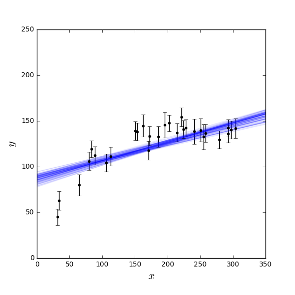
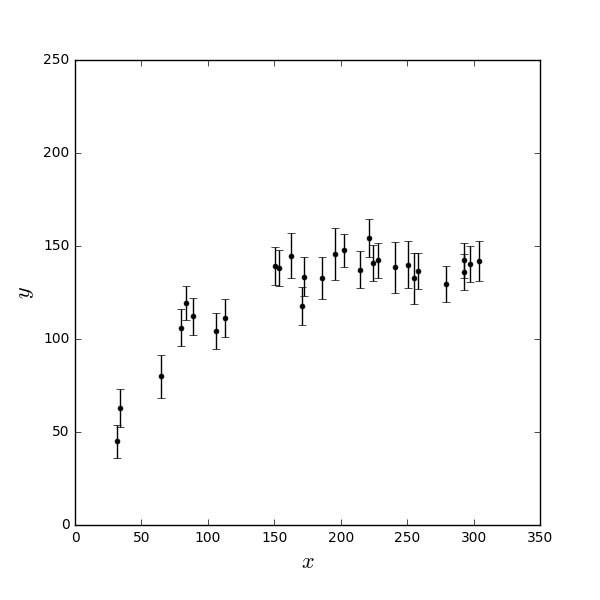
Some of the approaches discussed below are similar in spirit to those used in frequentism, so we'll work with an example that fits easily into both frequentist and Bayesian paradigms, namely classical least squares. So, imagine we have a data set like this:

Specifically, we'll assume that

• we have precisely known $x$ values,
• we have precisely known, Gaussian uncertainties on $y$ given $x$,
• we're (at first) fitting a linear model, $\bar{y}(x)=b+mx$, and
• priors on $b$ and $m$ will be Uniform over the real line.

In the language we've been using,

• $x_i$ and $\sigma_i$ (the Gaussian uncertainty on $y_i$) are known perfectly; $i=1,2,\ldots,n$ data points
• $m \sim \mathrm{Uniform}(-\infty,\infty)$
• $b \sim \mathrm{Uniform}(-\infty,\infty)$
• $\eta_i = b+mx_i$
• $y_i \sim \mathrm{Normal}(\eta_i, \sigma_i)$

To be explicit, the likelihood and posterior here are (up to a constant)

$p(\{y_i\}|m,b) \propto p(m,b|\{y_i\}) \propto e^{-\chi^2(m,b)/2}$,

with $\chi^2(m,b) = \sum_i \frac{(b+mx_i - y_i)^2}{\sigma_i^2}$ the classical $\chi^2$ statistic.$^1$

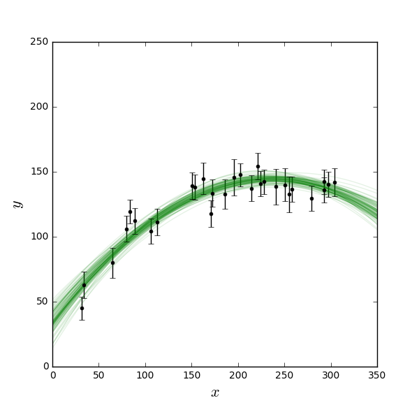
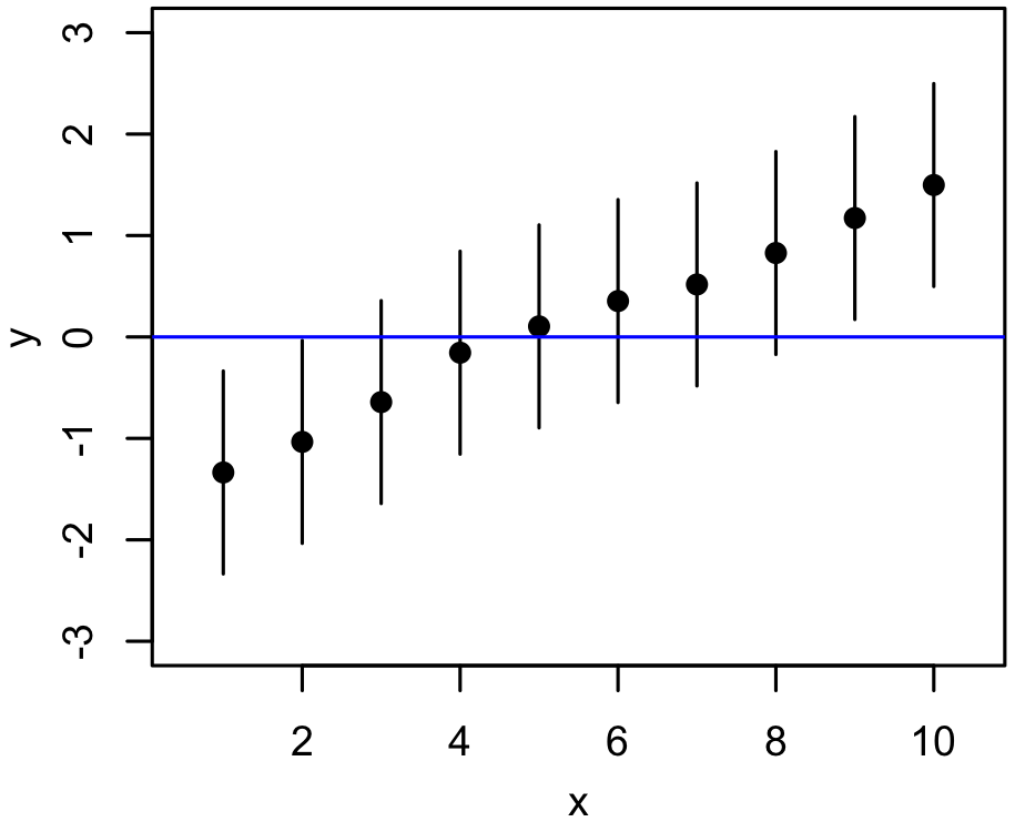
We've already seen one qualitative test in the Bayes' Law notes, namely visually comparing the data to mock drawn from the posterior. That would be a little more cumbersome in this case (which is not to say it wouldn't be worthwhile), but a simpler alternative might be to compare model curves from the posterior - without additionally drawing mock data from the sampling distribution - to the data plus "error bars". That might look like this figure:

If, as we are forced to in this case, we accept the error bars shown to be a Gaussian description of the sampling distribution for each data point, this might already look not-so-great for the linear model - quite a few of the points apear discrepant from the locus of model lines. But is it really worse than we should expect based on the randomness inherent in the generative model? Below, we'll look at ways to be more quantitative about this.

Frequentist Hypothesis Testing

Let $\hat{\chi}^2=\chi^2(\hat{m},\hat{b})$ be the minimum $\chi^2$ achievable for a given data set, and $\hat{m}$ and $\hat{b}$ be the corresponding (best-fitting) parameter values, i.e those that maximize the likelihood and posterior.

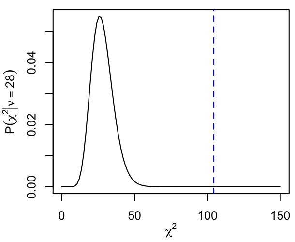
The classical approach is to test whether the data are consistent with predictions of this model, with parameters $\hat{m}$ and $\hat{b}$ (and all of the hidden assumptions about fixed/known $x_i$ and $\sigma_i$). Due to all of the liner/Gaussian assumptions in the model, this can be done in a relatively simple way. Namely, the predicted distribution over data sets of the minimum possible $\chi^2(m,b)$ should follow a $\chi^2_\nu$ distribution,$^2$ where $\nu=N_\mathrm{data}-N_\mathrm{parameters}$ (in this case, $N_\mathrm{data}-2$) is called the number of degrees of freedom.

Hence, the frequentist $\chi^2$ test looks at whether $\hat{\chi}^2$ is consistent with the distribution predicted by the best-fitting parameters. If not, it's unlikely that our data came from the assumed model with those parameter values, and since they were the best option, it's unlikley that the data came from the assumed model at all.

In our example, the value of $\hat{\chi}^2$ turns out to be $\approx104$, which doesn't look good in light of the expectation.

We refer to the integrated $\chi^2_\nu$ probability to the right of our measured $\hat{\chi}^2$, $P(\chi^2\geq\hat{\chi}^2|\nu)$, as the p-value or significance. In this case, it is $\sim10^{-10}$. In other words, the probability of a random data set produced by our assumed model with its best parameter values (called the "null hypothesis") resulting in a $\hat{\chi}^2$ value at least as extreme as the one we got is staggeringly small.

The p-value is not the probability of the model $(m,b)$ being true (remember, this is a non-Bayesian approach). Like the sampling distribution from which it is derived, it characterizes the probability of getting the data given the assumed model and its estimated parameters.

In our example, the result of a classical hypothesis test is of the following form:

"We reject the null hypothesis at the $p$ significance level"

(on the grounds that it inadequately explains the data).

Practical $\chi^2$ Testing

We can compute the p-value assuming a $\chi^2_\nu$ distribution using scipy.stats easily:

import scipy.stats as st
pvalue = st.chi2.sf(chisq_min, nu)

Here the sf function is shorthand for 1 minus the CDF, which is the integral we want.

The "reduced chi-squared", $\hat{\chi}^2_{R} = \hat{\chi}^2 / \nu$, is often used as a quick and dirty assessment of the goodness of fit.$^3$ The logic is that, since the $\chi^2_\nu$ distribution becomes relatively skinny for large $\nu$, and since its mean is $\nu$, $\hat{\chi}^2_{R}$ should be "close to 1". This is clearly a less robust statement than one based on a p-value.

Beyond $\chi^2$

One can devise frequentist tests that use statistics other than $\hat{\chi}^2$, for situations that don't merit all of the assumptions of the least squares case, but the basic logic is the same: if the model with the best fitting parameters is unlikley to produce the observed data then it is suspect.

The general approach is this: from our model with its best-fitting parameters, we generate a large number of mock data sets. We then compute some function of a data set, called a test statistic, on each of the mock data sets, and compare this distribution of values with the test statistic computed from the real data.

Since the first Bayesian approach we discuss below is a modification of this one, we won't go into it further. But note that the $\chi^2$ test fits into this paradigm as a special case. That is, under the linear/Gaussian assumptions, the distribution of our test statistic, $\hat{\chi}^2$, can be proven to be the $\chi^2$ distribution used above - there is no need to numerically evaluate the test statistic distribution by generating and analyzing mock data in this special case.

Bayesian Hypothesis Testing

In the Bayes' Law notes, we introduced the idea of comparing the data to posterior predictions of the model, i.e. mock data generated from the posterior distribution. The logic here is similar to that of the frequentist test: we want to see whether the fitted model can produce data that look like ours. However, instead of only looking at data generated from the "best-fitting" parameters, the Bayesian approach accounts for posterior uncertainty by generating mock (or replica) data from parameters sampled from the posterior distribution.

Apart from this distinction, one can similarly define a suitable test statistic, and compare its value as computed from the real data with the posterior predictive distribution computed from the replica data. In general, we are free to design our test statistic to focus on whatever aspect of the data that we want the model to fit well.

To reiterate, the logic behind posterior predictive model checking is:

• If our model is the true one, then replica data generated by it should in some sense resemble the one dataset we have.
• Because the data set may be high dimensional, it's convenient to encode "resemblance" through a scalar summary, $T(\mathrm{data})$, computed on a real or replica data set.
• The distribution of $T$, accounting for the sampling distribution and posterior uncertainty of the model parameters, can be computed using the generative model.
• If the real data set was not generated from our model, then its summary may be an outlier from the distribution of summaries computed from replica datasets.

Note the "may" in the last bullet. If our value of $T$ from the real data turns out to be unlikely under the model, it doesn't necessarily mean that the model is wrong... just that our value of $T$ from the real data is unlikely under the model. Unlikely things happen! This is a weakness of the approach shared with frequentist hypothesis testing generally, and motivates the use of model comparison (that is, explicitly asking whether one model is more likely than another), which we discuss more below. Nevertheless, posterior predictive checks are useful and relatively simple.

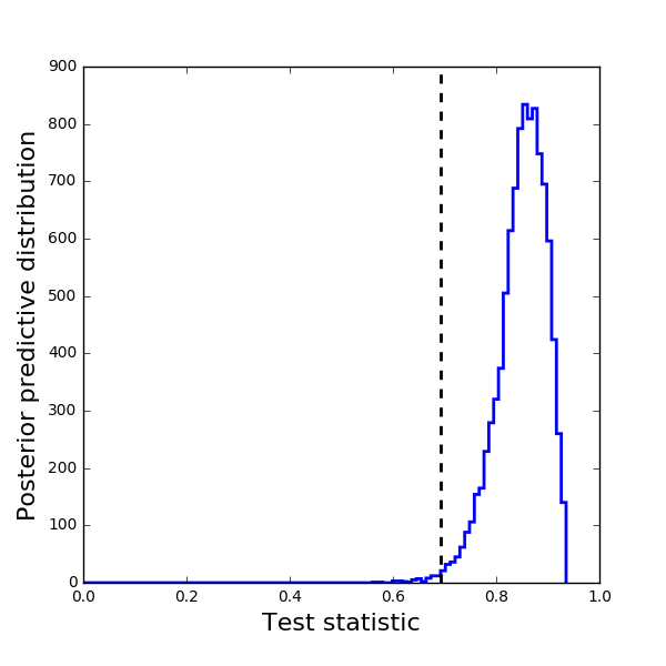
For our example, we might adopt the Pearson Correlation, $r_{12}$, as a test statistic.

$T(x,y) = r_{12} = \frac{\sum_i (x_i - \bar{x})(y_i - \bar{y})}{\left[ \sum_i (x_i - \bar{x})^2 \sum_i (y_i - \bar{y})^2 \right]^{1/2}}$

For each one of many posterior samples, we draw a replica dataset from the sampling distribution, and compute $T(x,y)$, building up a histogram of $T$. Compared with this distribution, the value of $T$ computed from the real data, $\hat{T}$, is a clear outlier, with $P(T>\hat{T}) \approx 99.4\%$.

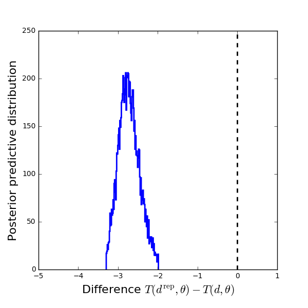
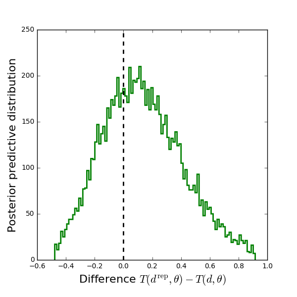
The test statistic used above was a function of the data alone. Test statistics can instead be functions of both the data and the parameters, in which case they are called discrepancy measures. The maximum log-likelihood is a common example, which in our example would reduce to the classical test, since the log-likelihood is $-\chi^2/2$. Using the log-likelihood, our predicted distribution looks like this, with zero simulated values of $T$ exceeding the discrepancy computed from the real data. (Recall that the frequentist p-value was of order $10^{-10}$; while $P(T>\hat{T})$ may be larger than this due to posterior uncertainty, which the p-value doesn't account for, it still seems entirely reasonable that none of our mere $10^4$ replica $T$ values exceeded $\hat{T}$.)

The two difference choices of test statistic thus lead to quantitatively different statements about how fit (or not) this model is. The former case might be vulnerable to our objection earlier - yes $\hat{T}$ looks unlikely, but every so often our real data set, as spit out by the sampling distribution, is going to be pretty unlikely. That argument, while technically still true, starts to sound a little absurd when we're talking about probabilities like $10^{-10}$, as with the second test. There isn't necessarily an ideal choice of test statistic in general; the log-likelihood is a common choice because of the analogy to $\chi^2$ and because it can be applied in any situation, while other test statistics might be superior in a situation where we don't expect any simple model to describe the data in detail, but want to find one that reproduces one particular aspect well.

Generalized Predictive Accuracy and "Information Criteria"

Based on the analyses above, we'd probably be uncomfortable with the quality of the fit provided by the linear model. How do we choose an alternative? One way to compare the fitness of models is to look at the second of our model evaluation questions: How accurately do they predict new data?

The idea behind generalized predictive accuracy is that we typically want a fit that works well with any potential data set, rather than just reproducing the one we have. In general, this means an "Occam's Razor"-like penalty for complexity should be involved, to avoid focusing on models that "over-fit" the data.

In our example, we might add a quadratic term to the model: $y = b + m x + q x^2$, which results in posterior model draws like those on the left below, and the predicted distribution of maximum log-likelihoods shown on the right.

Now the test statistic computed from the real data is comfortably within the predicted distribution, which seems like an improvement. However, we generically expect this kind of improvement whenever we add flexibility to a model (at least and especially because we chose the quadratic model based on looking at how the data and the linear model differed), so how do we quantitatively decide whether the additional parameter is justified?

The gold standard for testing predictive accuracy is to get more data, and compare them with the predictions. Short of that, the best option is cross-validation: fitting a model on many random subsets of the data and seeing how well it describes the complementary "out of sample" subsets. (This method is ubiquitous in machine learning, where accurate out-of-sample prediction is usually the goal.)

Short of exhaustive cross-validation, a number of information criteria exist that (asymptotically) relate to generalized predictive accuracy. These have the advantage of being relatively quick to calculate from the results of a fit - either a maximum likelihood estimate or a set of posterior samples - and include a penalty for models with greater freedom. Information criteria that you might come across include the

• Akaike information criterion (AIC)
• Deviance information criterion (DIC)
• Watanabe-Akaike information criterion (WAIC)

Of these, the DIC has the advantage of being compatible with Bayesian analysis (unlike AIC), and not requiring the data to be cleanly separable into conditionally independent subsets (unlike WAIC). It's defined as

$\mathrm{DIC} = D(\theta^\ast) + 2p_D = \langle D(\theta) \rangle + p_D; \quad p_D = \langle D(\theta) \rangle - D(\theta^\ast)$

where $D(\theta)=-2\log P(\mathrm{data}|\mathrm{params})$ and the average $\langle\rangle$ is over the posterior distribution. Here $\theta^\ast$ is some estimate of the center of the posterior, often taken to be the mean, $\langle\theta\rangle$, though in principle it could e.g. be the mode instead. The quantity $p_D$ is called the effective number of free parameters, and approximates the number of parameters that are primarily constrained by the data rather than by their priors; this may not be obvious from the definition above, but in practice it works out surprisingly well. Thus, while other information criteria include a term proportional to the total number of fitted model parameters in order to penalize more complex models, the DIC doesn't necessarily count unconstrained nuisance parameters that exist only to marginalize out systematic uncertainty towards this penalty.

Note that for all of these information criteria, a lower value is preferable (larger likelihood and/or less model complexity). A somewhat motivated scale for interpreting differences in IC exists (named for Jeffreys):

$$e^{(\mathrm{IC}_1-\mathrm{IC}_2)/2}$$	Strength of evidence for model 2
$<1$	Negative
$1$-$3$	Barely worth mentioning
$3$-$10$	Substantial
$10$-$30$	Strong
$30$-$100$	Very strong
$>100$	Decisive

Because it can be computed directly from posterior samples, the DIC is a fairly common alternative to the Bayesian evidence for quick-and-dirty model selection, if we can't be bothered to compute the evidence specially.

Exercise: Priors and the DIC

Say our model has 1 parameter, $\theta$, and the likelihood is a unit width Gaussian centered on $\theta=0$ with peak value $L_{\rm max}$.

For each of the priors on $\theta$ below, (a) sketch the likelihood and prior as a function of theta, (b) roughly approximate the DIC and $p_D$ for that model (just well enough for a qualitative comparison between the models).

1. $p(\theta|H_1)$ uniform on $[-1,+1]$
2. $p(\theta|H_2)$ uniform on $[-100,+100]$
3. $p(\theta|H_3)$ uniform on $[+3,+5]$

Recall: $\mathrm{DIC} = D(\langle\theta\rangle) + 2p_D; \quad p_D = \langle D(\theta) \rangle - D(\langle\theta\rangle)$

Solutions at the end of the notebook.

DIC exercise: comments

1. Models that are less prescriptive (in terms of their priors) are penalized in the DIC (models 1 vs 2).

2. However, there is a limit to this penalty. As the prior becomes less prescriptive, we get the penalty associated with "one more free parameter", and that's all.

3. Sufficiently large improvements to the likelihood will overcome the penalty (models 3 vs 2).

Bayesian Model Comparison

What about the third model evaluation question: How probable are our competing models in the light of the data? This question cannot be asked in classical statistics, where only data have probability distributions. However, Bayes theorem gives us a framework for assessing relative model probabilities that naturally includes Occam's razor.

Recall that we can write Bayes' Law for inference on parameters $\theta$ given a model $H$ and data $D$ as

$P(\theta|D,H)=\frac{P(D|\theta,H)P(\theta|H)}{P(D|H)}$.

Analogously, we can do inference on models within some space of possible models, $\Omega$;

$P(H|D,\Omega)=\frac{P(D|H,\Omega)P(H|\Omega)}{P(D|\Omega)}$.

Again, remember that $H$ includes all aspects of specifying the model, including our prior PDF assignments. Everything here has a straightforward analogy to the parameter inference that you're familiar with, so

• $P(H)$ is a prior probability over models;
• $P(D|H)=\int P(D|\theta,H) \, p(\theta|H) \, d\theta$ is the evidence, which previously appeared in the denominator for parameter inference but now takes on the role that the sampling distribution had; and
• $P(D|\Omega)$ is a new normalizing factor, which we will normally ignore (just as we didn't worry about the evidence when doing only parameter inference).

To compare models within the space $\Omega$, we would look at the ratio of their posterior probabilities,

$\frac{P(H_2|D)}{P(H_1|D)}=\frac{P(D|H_2)\,P(H_2)}{P(D|H_1)\,P(H_1)}$.

which simply requires us to

• assign meaningful priors to models,
• assign meaningful priors to parameters, and
• calculate the evidence integral.

The Bayesian approach is qualitatively different from other model assessments discussed above. While they focused primarily on prediction accuracy, here we simply apply Bayes' Law at the level of the model as a whole, with the evidence updating our prior knowledge into a posterior probability. There are no inherent mathematical limitations to this procedure, in contrast to various other hypothesis tests that are only valid under certain assumptions (such as the models being nested, e.g. the classical $F$ test for comparing $\chi^2$ values). Any two models, no matter how fundamentally different, can be compared with this technique.

Exercise: Priors and the evidence

Again, consider a model with 1 parameter, $\theta$, and a likelihood that works out to be a unit width Gaussian centered on $\theta=0$ with peak value $L_{\rm max}$.

For each of the priors on $\theta$ below, (a) sketch the likelihood and prior as a function of theta, (b) roughly approximate the evidence for that model (just well enough for a qualitative comparison between the models).

1. $p(\theta|H_1)$ uniform on $[-1,+1]$
2. $p(\theta|H_2)$ uniform on $[-100,+100]$
3. $p(\theta|H_3)$ uniform on $[+3,+5]$

Recall: $P(D|H)=\int P(D|\theta,H) \, p(\theta|H) \, d\theta$.

Solutions at the end of the notebook.

Evidence exercise: comments

1. Models that are less prescriptive (in terms of their priors on parameters) are penalized in the evidence. This is a feature, although it means we need to put real thought into those priors, instead of mindlessly choosing something wide and uniform.

2. The evidence can be made arbitrarily small by increasing the prior volume; comparing evidences is therefore more conservative than focusing on the best achievable likelihood ($L_{\rm max}$) alone.

3. Still, the evidence is only linearly sensitive to prior volume. For typical models where the likelihood is exponentially sensitive to how closely the model reproduces the data (e.g. $e^{-\chi^2/2}$), achieving a better fit will make a big difference

Bayes factors

A form of Bayesian hypothesis testing that you might encounter is model comparison with the "evidence ratio" or "odds ratio" or "Bayes Factor",

$R = \frac{P(D|H_2)}{P(D|H_1)}$.

Notice that this is simply the ratio of posterior probabilities if the prior probabilities of $H_1$ and $H_2$ are equal. This assumption is often not particularly easy to justify, tempting though it might be. A more practical way to interpret the Bayes factor is to note that it updates the model prior ratio into the posterior ratio,

$\frac{P(H_2|D)}{P(H_1|D)}=\frac{P(H_2)}{P(H_1)} R$.

The same Jeffreys scale used to interpret the information criteria can be used to interpret evidence ratios:

$R$	Strength of evidence for model 2
$<1$	Negative
1-3	Barely worth mentioning
3-10	Substantial
10-30	Strong
30-100	Very strong
$>100$	Decisive

Returning to our example data set and models, we can compute the evidence for the linear and quadratic models, and form the odds ratio, $R$. (The specific uniform priors used in these calculations have been lost to time, but see comment 3 on the exercise above.)

log Evidence for Straight Line Model: -157.2
log Evidence for Quadratic Model: -120.7
Evidence ratio in favor of the Quadratic Model:
  7e15 to 1

The 26 unit difference in log evidence between the two models translates to a huge odds ratio in favour of the quadratic model. So, whatever method we choose in this case, it seems that we would be justified in discarding the linear model in favor of the quadratic one. Of course, this doesn't prove that the data did come from a quadratic model (they didn't), just that they are more consistent with that hypothesis than a linear one.

Calculating the evidence

Estimates of the evidence directly calculated from Markov chains produced for parameter inference are generally not reliable, since they don't cover the parameter space efficiently. An quick and dirty alternative is the Bayesian Information Criterion (BIC), which is an approximation of the evidence in the limit that that the data points greatly outnumber the parameters, and the priors are uninformative. However, the DIC is now a more common/recommended option for this situation, since it actually uses the information from the MCMC samples rather than just the maximum-likelihood point, as the BIC does.

A better choice, if feasible, is to use non-MCMC Bayesian methods such as nested sampling that can both estimate the evidence and produce samples suitable for our usual parameter inference (see notes on More Samplers).

Concluding remarks

There was a lot to digest in these notes - lots of different approaches one could take to accomplish somewhat different goals. We'll leave you with two bits of common sense that should not be forgotten amongst all of this:

"Acceptable" is not the same as "not stupid"

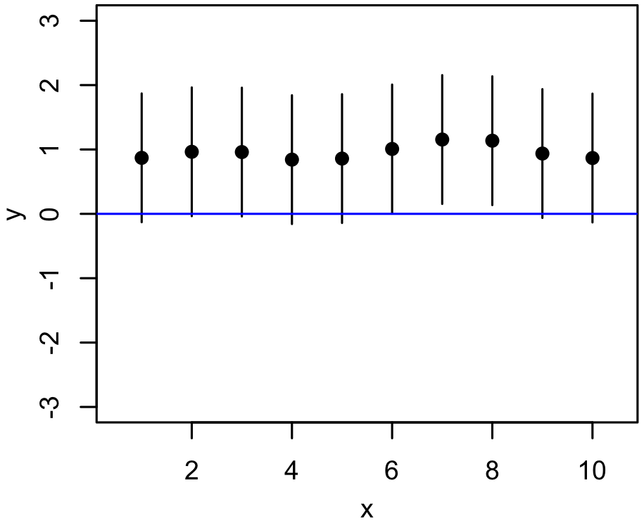
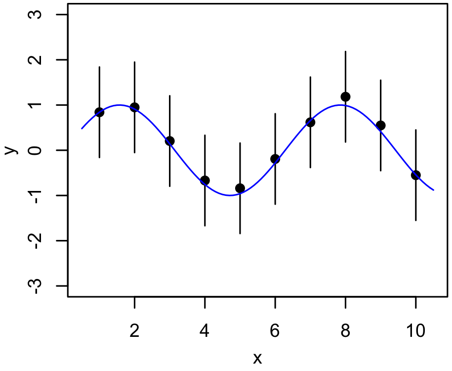
This is a reminder that model/fit evaluation can never be something completely automatic that we disconnect our brains from. If we did a $\chi^2$-type fit evaluation, the data and model fits below might both be "acceptable", but each one strongly suggests that the assumptions we made about the sampling distribution (independence of data points, size of the uncertainties) or the model were incorrect.

The converse situation is probably more common - say your model for the profile of an uninteresting (to your science) emission line is known to be a little wonky, such that a fit to your spectral data will leave some large residuals that prevent it from being formally acceptable, while producing no other ill effects (an important caveat). Sure it would be nice if someone fixed the model, but should you go down a rabbit hole of comparing the evidence among a dozen slightly tweaked models? Probably not.

"Acceptable" and "not stupid" are also distinct from "best suited for a specific purpose"

Or, consider the following. If a non-constant model for these data would be groundbreaking, proving that everything we thought we knew about the Universe was wrong!!!, then a responsible scientist would emphasize that the constant model is adequate to describe the data (while still definitely noting that the data are darned suggestive).$^4$

On the other hand, if these data represent a correction to our instrument's gain, and especially if we have reason to expect that a linear correction may be needed, we might go ahead and change to a linear model even though the data don't conclusively disfavor a constant model. (That is, we might put ourselves in the same situation as the right-hand figure above, but deliberately - because we were just looking for a function that describes the data and weren't overly concerned with it being fundamentally correct.)

Endnotes

Note 1

With deepest apologies, we will follow the terrible practice of using the symbol $\chi^2$ to refer to both this function and to the chi-square probability distribution, $\chi^2_\nu$.

Note 2

See Note 1.

Note 3

Believe it or not, the notation $\chi^2_\nu$ is often used for the reduced chi-squared, thus negating the silver lining to Note 1 you may have identified.

Note 4

Bets on whether this would be the messaging in practice? Anyone?

Exercise solution - DIC

It should be possible to reason through a qualitative comparison of the 3 proposed models, but, for completeness, the following code does an actual quantitative comparison.

import numpy as np
import scipy.stats as st
def DIC_thingy(lower, upper):
    y = st.truncnorm.rvs(lower, upper, size=100000)
    av_of_D = np.mean(-2.0*st.norm.logpdf(y))
    D_of_av = -2.0*st.norm.logpdf( np.mean(y) )
    pD = av_of_D - D_of_av
    DIC = D_of_av + 2*pD
    return pD, DIC

print(DIC_thingy(-1.0, 1.0))
print(DIC_thingy(-100.0, 100.0))
print(DIC_thingy(3.0, 5.0))

(0.2929629758172452, 2.4238064854775434)
(0.9976504087908931, 3.8331933598331265)
(0.06958630683580047, 12.749912636788213)

Exercise solution - evidence

Once again, one can reason out a qualitative comparison without doing the calculations (more easily than with the DIC, in fact). But the code below will also do it.

def Evidence_thingy(lower, upper):
    return (st.norm.cdf(upper) - st.norm.cdf(lower)) / (upper - lower)

print(Evidence_thingy(-1.0, 1.0))
print(Evidence_thingy(-100.0, 100.0))
print(Evidence_thingy(3.0, 5.0))

0.3413447460685429
0.005
0.00067480569002909