Notes: Monte Carlo Sampling

In which we will

• Review the motivation for doing MC sampling in inference
• Look at the basic principles and methods of sampling
• Dig into Markov Chain Monte Carlo and two of the workhorse algorithms

Motivation: why sample?

In exploring the consequences of Bayes' Law so far, we've restricted ourselves to inferences with analytic solutions and low-dimensional parameter spaces. Needless to say, these are not typical use cases for us.

In general, we will not have a convenient analytical solution, and evaluating the posterior throughout the entire parameter space will be too costly. We want to focus resources on mapping the posterior where it is non-tiny. Generating samples from the posterior itself, or a similar PDF, accomplishes this.

Sampling and numerical integration

In principle, given samples from the posterior, we could estimate the density at any point using some form of kernel density estimator. However, as you saw in the notes on credible regions, the results we report are usually based on marginal posteriors over 1 or 2 parameters. In other words, we are ultimately interested in integrals of the posterior. These integrals can also be computed from a set of posterior samples using Monte Carlo integration, and in general the number of samples we need to accurately estimate the 1D and/or 2D marginal posteriors is far fewer than we would need to accurately estimate the full-dimensional posterior density.

The essence of MC integration is as follows. Given any integrand, $f(x)$, factor $f$ into a product, $p(x)w(x)$, in which one term ($p$) is a PDF that is non-zero over the domain of integration. Draw $n$ samples from $p(x)$, and evaluate $w(x)$ at each of these $x_i$, $i=1,\ldots,n$. The integral can then be approximated as

$\int f(x) \, dx = \int w(x) \, p(x) \, dx \approx \frac{1}{n}\sum_i w(x_i)$; $x_i \sim p$.

This approximation becomes exact in the limit $n\rightarrow\infty$ no matter what $p$ we choose, provided that it is non-zero everywhere between the limits of integration that $w(x)$ is non-zero. However, how quickly the average converges to the correct integral (what $n$ needs to be) does depend on the choice of $p$.

How does this help us? Let's imagine we have a clever way of sampling from the posterior distribution, whatever it happens to be. If the posterior is 1D to begin with, we can simply estimate the posterior density based on the density of samples, e.g. by making a histogram, and find our best value and credible interval from there. But if the posterior is multi-dimensional, we will need to integrate it down to get a 1D marginal posterior for a single parameter. We can do that by simplemindedly using the approximation above, with $p$ being the posterior itself, and $w=1$. That is, if $\theta$ is the parameter we care about and $\phi$ are those we want to integrate out,

$p(\theta|\mathrm{data}) = \int d\phi \, p(\theta,\phi|\mathrm{data}) = \int d\phi \, p(\theta,\phi|\mathrm{data})\times 1 \approx \frac{1}{n}\sum_{i:\theta_i=\theta} 1$; $\theta_i,\phi_i \sim p$.

This might look like it will be 1 all the time, but remember that the integral here is at a fixed value of $\theta$. So, the corresponding sum is only over samples with that value of $\theta$, and there are probably fewer than $n$ of them. (If it's still confusing, imagine modifying the above to integrate over both $\phi$ and $\theta$ - that certainly should return 1, since the posterior is normalized. Now, imagine straightforwardly removing the integral over $\theta$.)

In practical terms, this means the that the correct procedure is the most straightforward thing one could imagine. If we have posterior samples, the way we estimate the 1D marginalized posterior of $\theta$ is to ignore all other parameters and simply make a histogram of the $\theta$ values from our samples, just like in the case where the posterior was 1D to begin with. Similarly, a 2D marginalized posterior would be estimated based on a 2D histogram made from the samples of just 2 parameters, regardless of what the other parameters are doing.

Note that MC integration will work for us even if we sample from some distribution other than the posterior itself, if we chose $w$ appropriately. There are algorithms tailored to both possibilities.

Simple Monte Carlo

We've already seen a natural and non-trivial factorization of the posterior, into a likelihood function and a prior PDF,

$p(\theta|\mathrm{data}) \propto p(\mathrm{data}|\theta)\,p(\theta)$.

Applying this in the MC integration context leads to the Simple Monte Carlo algorithm:

while we want more samples
    draw theta from p(theta)
    compute weight = p(data|theta)
    store theta and weight

Obtaining marginal posterior distribution(s) for $\theta$ then reduces to constructing weighted histograms of the samples. This is hardly different from the case considered above, where the weights happened to be equal.

SMC is indeed simple (as long as the prior is simple to draw from), but if the priors are not very informative then it can be very inefficient, wasting many likelihood evaluations where the posterior is small. Indeed, if all the priors are uniform, SMC is no more efficient than evaluating the posterior over a grid. However, refinements of this approach lead to some of the advanced algorithms we'll cover later.

Importance weighting/importance sampling

Here is another straightforward application of the basic premise of MC integration. Say we have already done an analysis in which we obtained samples from some $p$, and the corresponding weights $w$, which together provide information about a posterior distribution. Now imagine that we want to incorporate a second data set into the inference. We can do this without generating more samples, by simply multiplying the weights with the likelihood associated with this second data set, and repeating whatever integrations we wanted to do (i.e., making new weighted histograms). This will work as long as the original samples span the domain over which the second likelihood is significantly non-zero, although it may leave us with "effectively" fewer samples (because the new weights for some of our samples are now very small).

Equivalently, we could leave the weights alone, but re-sample from our original list of samples with probabilities proportional to the second likelihood.

Random number generation

Before diving any further into the algorithms used for Bayesian analysis, it's worth reviewing the more fundamental approaches to generating pseudorandom numbers from some distribution. We won't normally use these procedures directly, but conceptually they play a role in the algorithms that we will use.

To begin with, let's get the terminology straight.

• Random: not deterministic; predictable only in the sense of following a PDF. Computer algorithms do not produce random numbers.

• Pseudorandom: not random, but "unpredictable enough" for practical purposes. The usual "random number generator" algorithms that are standard, e.g. in numpy, actually produce pseudorandom sequences. Generally, these approximate the uniform distribution on the interval [0,1). These sequences depend on an initial state, called a seed, such that they are completely predictable based on the seed. Hence notebooks or calculations that use pseudorandomness, but are intended to be reproducible, will explicitly set the seed of the random number generator at the outset. (We could have done that throughout this course to provide tutorial outputs that should exactly match yours, but chose not to out of laziness.)

• Quasirandom: not random, and "more predicable" in human terms than pseudorandom. A quasirandom sequence can therefore converge to the target PDF (in the sense of sampling it evenly and having the right mean, standard deviation, etc.) more quickly than a truly random or pseudorandom. This can make them very useful for MC integration generally, although less so for our purposes, since we want to generate random-seeming samples as well as integrations. For example, one classic quasirandom sequence goes: $1/2, 1/4, 3/4, 1/8, 7/8, 3/8, 5/8, \ldots$

In this section, we assume that we have a reliable source of uniform pseudorandom numbers, and need to transform them into samples from some other PDF. (In days past, we would caution you about the fact that these generators eventually repeat themselves - that is, the sequences are periodic - but the standard algorithms in numpy and similar packages have vastly longer periods than those that used to be the default for programmers in C and Fortran. Still, if you are generating initial conditions for some huge N-body simulation, this would be something to watch out for.)

Inverse transform method

Recall the definition of the CDF (and it's inverse, $F^{-1}$, the quantile function),

$F(x') = P(x \leq x') = \int_{-\infty}^{x'} p(t)\,dt$.

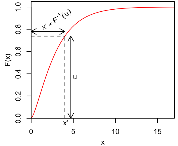
If $x$ follows the distribution $p$, then, by definition, $F(x)$ is uniformly distributed on [0,1]. If $F^{-1}$ is easy to evaluate, we can use this straightforwardly,

while we want more samples
    draw u from Uniform(0,1)
    compute x = F_inverse(u)
    store x

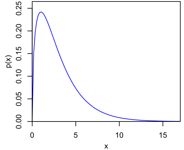
The resulting x will follow the distribution whose quantile function is $F^{-1}$, which is exactly what we want. This is illustrated in the plots below, where the left figure shows some PDF, and the right shows the corresponding CDF, with a uniform draw along the $y$ axis leading to the selection of a quantile along the $x$ axis. Intuitively, our samples of $x$ will cluster most densely where the CDF is steep (i.e., where its derivative, the PDF, is large).

Example: the exponential distribution

This distribution has $p(x)=\lambda e^{-\lambda x}$ and $F(x)=1-e^{-\lambda x}$ for $x\geq0$.

The quantile function is, therefore, $F^{-1}(\mathcal{P}) = -\frac{\ln(1-\mathcal{P})}{\lambda}$.

Let's go ahead and implement an exponential number generator in code.

# import stuff
import matplotlib
matplotlib.use('TkAgg')
import matplotlib.pyplot as plt
plt.rc('text', usetex=True)
plt.rcParams['xtick.labelsize'] = 'x-large'
plt.rcParams['ytick.labelsize'] = 'x-large'
import numpy as np
%matplotlib inline

def inv_trans_expn(mean=1.0, number=1):
    '''
    Generate `number` random draws from an exponential distribution with mean parameter `mean`.
    '''
    u = np.random.rand(number)
    x = -np.log(1.0 - u) / mean
    return x

Here's how a normalized histogram of such numbers compares to the exponential PDF:

lam = 1.0 # choose a mean
x = inv_trans_expn(lam, 10000)
hist = plt.hist(x, bins=50, density=True);
xs = np.linspace(0.0, 10.0/lam, 100)
pdf = lam * np.exp(-lam*xs)
plt.plot(xs, pdf, lw=2);
plt.xlabel(r'$x$', fontsize='x-large');
plt.ylabel(r'$p(x)$', fontsize='x-large');

Rejection sampling

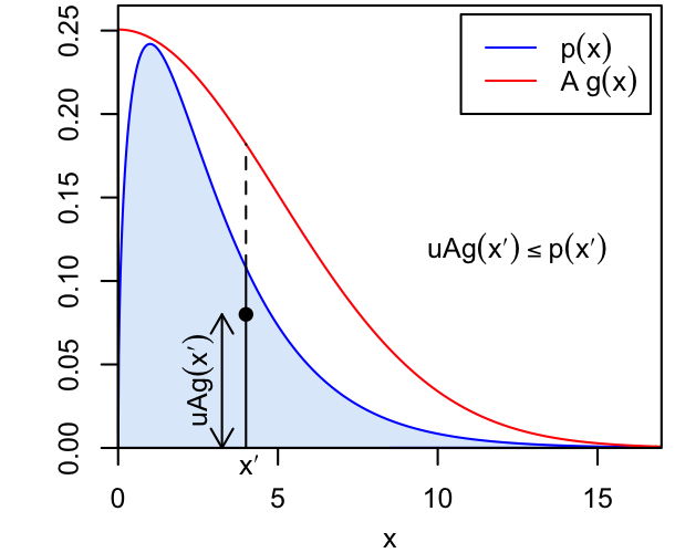
For this method, we need to define an envelope function which everywhere exceeds the target PDF, $p(x)$. We'll want this function to be non-negative, but it need not be normalized. Let this be $Ag(x)$ where $A$ is a scaling factor and $g(x)$ is a PDF we can already sample from.

The algorithm is

while we want more samples
    draw x from g
    draw u from Uniform(0,1)
    if u <= p(x)/(A*g(x)), keep the sample x
    otherwise, reject (do not store) x

Visually, this corresponds to drawing points that uniformly fill in the area under $Ag(x)$, then throwing away all those that are not also under $p(x)$, such that we ultimately sample uniformly under $p(x)$. The $x$ values of these remaining points thus automatically have the right distribution. Note that we will need to traverse the loop more times than the number of samples we want, and that the rejection rate naturally depends on how closely $Ag(x)$ resembles $p(x)$.

Markov Chain Monte Carlo

Both of the algorithms above generate independent sequences of random numbers. That is, putting aside the essentially deterministic nature of the pseudorandom generators underneath, each sample is independent of the samples before it. This is a nice feature. However, neither algorithm is immediately useful for a general PDF; we would need to laboriously construct a quantile function or an efficient envelope function.

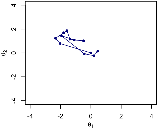
There are algorithms that work straightforwardly for more general PDFs, but come with the disadvantage that samples are not independent of one another, they are correlated sequences. In the class of algorithms we are concerned with now, each sample has a direct dependence on the immediately preceding one, making the sequence a kind of random walk, technically known as a Markov process. Hence the name Markov Chain Monte Carlo (MCMC).$^1$

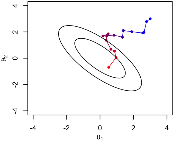
Here is an illustration of such a Markov chain in a 2-dimensional space, with just a few samples in it.

In order for a Markov chain to be interpreted as samples from a PDF, the transition kernel (the probability of moving from one point in the parameter space to another) must satisfy a few requirements.

• Detailed balance: any transition must be reversible; the probability of being at $x$ and moving to $y$ must equal the probability of being at $y$ and moving to $x$.
• Ergodicity: it must be possible, in principle, for the chain to reach any point where the PDF is non-zero in finite time, as well as to return in finite time to a point it has already visited; however, the process may not be periodic.

Why does this work?

The proof may not be not particularly intuitive (it's by induction rather than deduction), but we'll sketch it out here. Let's start by assuming that our chain does indeed sample from a target distribution, $p$. The probability of an arbitrary point from this chain being located at $y$, marginalizing over the possible immediately preceding points, $x$, is,

$p(y) = \int dx \, p(x) \, T(y|x)$,

where $T(y|x)$ is the transition probability of a step from $x$ to $y$. Note that, according to our assumption, $p(y)$ and $p(x)$ refer to the posterior PDF, not any old $p$. The transition kernel is sometimes written $T(y,x)$ (or $T(x,y)$, or $T(y;x)$, etc.), but by definition it must have the properties of a probability distribution over $y$ (normalization in particular), so we find it helpful to write it as $T(y|x)$.

If we have detailed balance, then $p(x)T(y|x) = p(y)T(x|y)$, and

$p(y) = p(y) \int dx \, T(x|y) = p(y)$.

So we have successfully proven that $1=1$. Huzzah!

The important point here is, of course, that we needed detailed balance in order to reach this unambiguously true statement, and conversely we would not have gotten there otherwise. In other words, both the PDFs in the expressions above can represent the target distribution only if we evolve the chain in a way that respects detailed balance.

Furthermore, "both the PDFs represent the target distribution" is a statement about the long-term behavior of the chain. We can see this in the fact that the PDFs in question are marginal probabilities. That is, they effectively correspond to picking a sample in the chain at random to look at. It categorically is not a statement about the short-term behavior of the chain. We might investigate that by writing down $p(y|x)$ - that is, by conditioning on the previous position - which explicitly reveals the random-walk nature of the chain. This doesn't mean that we can't use all the steps in a chain to make inferences, but, as we'll see below, we do need enough samples that the long-term behavior is expressed.

You'll notice that we didn't explicitly invoke the requirement of ergodicity above, but its necessity is hopefully not implausible. If the chain cannot, even with infinite time, explore some part of the parameter space where the target PDF is non-zero, then we clearly can't say that it samples from that PDF.

General features of monte carlo Markov chains in practice

There are two features of MCMC that we will be very concerned with a bit later, when we need to decide whether the algorithm is behaving well for us.

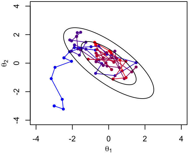
First, a chain will take some number of steps to converge to the target distribution. This is most clear if the chain starts somewhere that the target PDF is small - it will take a while to random-walk to the region where most of the probability is located. The plots below show the 1st hundred and 2nd hundred steps of an example chain, color coded by time/iteration number (blue$\rightarrow$red); ellipses show iso-probability contours in the usual way.

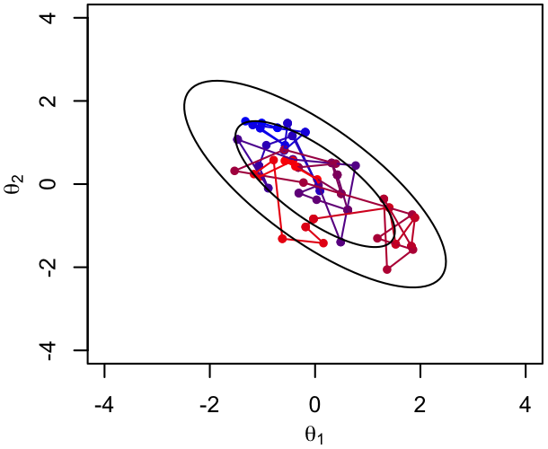The second feature is just the fact, clear in the illustration above, that the samples are correlated with one another. We need to remember that a chain of a given length contains less information about the target PDF than the same number of independent samples would.

The main practical consequence of this is that using MCMC is not a fully automatic process. We will need to cast our eyes over the resulting chains to verify that they have, indeed, converged to a sensible distribution, and that we have a reasonable number of samples given the degree of correlation. This is a subject we'll return to after discussing how to generate such a chain to begin with.

In these notes, we'll look at two such MCMC algorithms.

(Conjugate) Gibbs sampling

Gibbs sampling is less an algorithm than a strategy. In essence, we replace the task of generating samples from a high-dimensional posterior, $p(\theta_1, \theta_2, \ldots, \theta_n|\mathrm{data})$, with the task of sampling in turn from a sequence of lower-dimensional conditional posterior distributions: $p(\theta_1|\theta_2, \ldots, \theta_n, \mathrm{data})$, $p(\theta_2|\theta_1, \theta_3, \ldots, \theta_n, \mathrm{data})$, ..., $p(\theta_n|\theta_1, \theta_2, \ldots, \mathrm{data})$. In pseudocode,

choose starting values for theta1, theta2, theta3, ...
while we want more samples
    sample theta1 from p(theta1 | theta2, theta3, ..., data)
    sample theta2 from p(theta2 | theta1, theta3, ..., data)
    ...
    store theta1, theta2, theta3, ...

Visually, this corresponds to taking steps through parameter space that are always parallel to one of the coordinate axes (though, e.g., updating two parameters at once, with the others fixed, would also be called Gibbs sampling). The order of updates can be either fixed or randomized, provided that every parameter does get updated sooner or later.

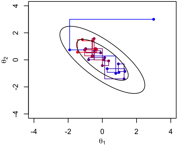Hopefully, it's intuitive that such a sequence converges to the multidimensional target PDF. By construction, the density of points in any of the conditional distributions will be correct. We just need the parameter not being conditioned on to have a chance to move around, and since we sample each parameter in turn, it has a chance to do so. More formally, as long as the individual-parameter updates satisfy detailed balance and the other requirements of MCMC, the sequence as a whole will also.

The decomposition used in Gibbs sampling is, of course, only helpful to the extent that sampling from the conditional posteriors is easier than from the full posterior. In general, this is not obviously the case. However, it can happen that one or more of the conditional posteriors is conjugate (see Bayes' Law notes), even if the full posterior is not. The corresponding update rule(s) then become very easy - we just need to sample from a standard PDF for which methods already exist, after computing the parameters of that distribution from the data and the fixed (conditioned-on) model parameters.

Granted, physical models, especially those involving nonlinear equations, don't always lend themselves to conjugacy. But, often enough, we are dealing with what you might call "descriptive" models, which tend to be built from simple functions and standard PDFs. In those cases, it's not so uncommon to have some conjugacies in the model. Since Gibbs sampling in these cases can be much more efficient than alternatives, it's worth knowing about this method as an option.

A classic non-trivial case where conjugate Gibbs can be used is for fitting a line to data, where both the $x$ and $y$ variables have some (normal) measurement error, including correlation between the $x$ and $y$ errors, and there is additional (normal) intrinsic scatter in $y$ for a given $x$. Classical least squares can't handle this, but the features above are hardly unusual in real-world problems.

Some packages that do Gibbs sampling

• JAGS the most general solution within the Python ecosystem, although the code itself must be installed (and can be used) outside of Python. The pyjags package provides an optional Python interface.
• BUGS is a similar, but lacks the optional Python interface.
• linmix is a specialized conjugate Gibbs sampler for univariate linear regression with heteroscedastic errors and intrinsic scatter (based on the IDL code linmix_err).
• LRGS is similar, but accomodates multivariate linear regression.
• BCGS is... probably not useful outside of the Vaccine Efficacy tutorial where you've already seen it, but is mentioned for completeness.

Metropolis-Hastings sampling

This algorithm can be thought of as an MCMC adaptation of rejection sampling. Unlike conjugate Gibbs, for which we only need to specify the posterior and a starting point in parameter space, here we need to additionally define a proposal distribution, $Q(y|x)$, giving the probability that we attempt to move the chain from $x$ to $y$.

If $p$ is the PDF we're trying to sample, the algorithm is then

choose a proposal distribution, Q
set x to an initial guess
compute p(x)
while we want more samples
    draw y from Q(y|x)
    compute p(y)
    draw u from Uniform(0,1)
    if u <= p(y)/p(x) * Q(x|y)/Q(y|x), set x=y
    otherwise, do not change x
    store x as a sample

Note that even if a step is rejected, we still keep a sample (the original state, without moving). The difficulty of finding a temptingly better point is important information!

In the algorithm above, the probability of accepting a step once it's proposed is

$\alpha(y,x) = \mathrm{min}\left[1, \frac{p(y)Q(x|y)}{p(x)Q(y|x)}\right]$

Let's look again at the requirement of detailed balance

the probability of being at $x$ and moving to $y$ must equal the probability of being at $y$ and moving to $x$

Here, the probability of being at $x$ and moving to $y$ is $p(x)\,Q(y|x)\,\alpha(y,x)$, where, remember,

• $p(x)$ is the target PDF (probability of being at $x$, if we're sampling properly)
• $Q(y|x)$ is the proposal distribution (probability of attempting a move to $y$ from $x$)
• $\alpha(y,x)$ is the probability of accepting that proposed move

Plugging in the definition of $\alpha$, we see that detailed balance is automatically satisfied!

$p(x) \, Q(y|x) \, \alpha(y,x) \equiv p(y) \, Q(x|y) \, \alpha(x,y)$

We still haven't said what the proposal distribution, $Q$, should be. In principle, it could be anything, so long as it's eventually possible to propose a move to anywhere the target PDF is non-zero. This makes it possible to use a tailored proposal distribution in cases where the target PDF is so complicated that we need to customize our algorithm to achieve convergence. However, in most cases, we instead use a more generic, translation-invariant proposal, with $Q(y|x)=Q\left(\left|y-x\right|\right)$. In this case, the proposal distribution drops out of the expression for the acceptance probability:

$\alpha(y,x) = \mathrm{min}\left[1, \frac{p(y)}{p(x)}\right]$.

In this case, we always accept a proposal to higher $p$, and sometimes accept one to lower $p$. This simplified version of the algorithm is called Metropolis sampling.

And yet, we still haven't managed to say what sort of function $Q$ should be. Obviously, we want our proposed steps to be large enough that we can traverse the target PDF, but not so big that every proposal is rejected. Arguably the simplest proposal to code is a multivariate Gaussian centered on the current position, but this has the disadvantage that the most likely proposals are very nearby. One can also choose distributions that make very short steps less likely, as in the blue curve below.

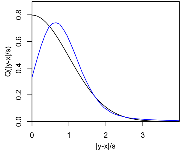Fairly generically, such distributions will have an overall scale (called $s$ in the figure above) for the distance of the proposed steps, which could be direction dependent. This scale can and should be tuned to give us a decent acceptance rate; this can be done automatically, though note that changing the proposal scale while the chain is running technically violates detailed balance.

And what acceptance rate would we ideally like? If every proposal is accepted, then we're probably not moving very far in parameter space with each step, and so our samples will be very correlated. But we do need to move! It's been said that an acceptance rate of 25% is somehow ideal, but really anything of this order is fine.

Conjugate Gibbs as a specialization of Metropolis-Hastings

Suppose we were somehow able to propose from the target PDF itself. Then the acceptance probability would be

$\alpha(y,x) = \mathrm{min}\left[1, \frac{p(y)Q(x|y)}{p(x)Q(y|x)}\right] = \mathrm{min}\left[1, \frac{p(y)p(x)}{p(x)p(y)}\right] = 1$,

and every step would be automatically accepted! This is essentially what's going on for each of the conditional posteriors in conjugate Gibbs sampling, which is why there is no accept/reject decision in that procedure. The same could be said of the trivial case where we have a target distribution that we can directly produce independent samples from.

The fact that we don't need to carefully tune a proposal distribution to get a good acceptance rate is one of the nice features of conjugate Gibbs. On the other hand, if there are strong parameter degeneracies, a well tuned (in multiple dimensions) Metropolis sampler can potentially be the more efficient way to explore parameter space.

Below is a comparison of the first 25 Metropolis iterations (left, reasonably but not ideally tuned) vs. the first 25 Gibbs transitions (right) for chains targeting a particular bivariate normal PDF. It's clear that the Gibbs sampler reaches the region of high probability much more quickly. On the other hand, the perpendicular nature of its steps could conceivably make it less efficient at accumulating samples once there, given the degeneracy of the two parameters shown.

Some packages that do Metropolis sampling

• PyMC, although this package has gotten so fancy and complex that we can't even find documentation on mere Metropolis sampling on the official website.
• LMC is a more basic alternative, which we are biased to think might be useful (especially if parallelization by MPI is natural for a given problem).
• As this is arguably the simplest MCMC algorithm, you can probably find many implementations, with various degrees of automated proposal distribution adaptation, by just searching the web.

Does it always work?

No! I don't know of any numerical procedures in this sphere that can be said to always work, with certainty. But it's easy to contrive a PDF that Gibbs sampling or Metropolis would fail to characterize, namely one with multiple, widely separated peaks that can't plausibly be random-walked between. We could tackle this with Metropolis-Hastings if we knew where the peaks were ahead of time and used a custom proposal distribution. But a Gibbs sampler would be dead in the water, unless the peaks were displaced along the Cartesian directions of the parameter space, and a Metropolis kernel with a reasonable proposal size to sample one peak would struggle to find its way to a different peak. (Ok, strictly speaking any of these algorithms would be fine after an infinite number of steps, but who wants to wait that long?)

So how can we be confident that we've mapped the whole PDF? Ideally, the structure of the model (or experience with similar analyses) would tell you whether multiple peaks are likely to exist. In full generality, we would need to exhaustively search the parameter space to be sure. Short of that, we could run many independent chains with widely separated starting points and see where they end up. (As you may know, this is also a generic issue in numerical optimization, nothing specific to MCMC.) If we do find that our PDF has multiple, widely separated peaks, there are other algorithms that will work better, which we will look at later on.

And isn't there a non-zero probability that our chain will run off to some low-probability region and stay there for an arbitrarily long time? Yes. Yes, there is. And it is equally arbitrarily unlikely for that to happen. Staggeringly unlikely. Floating point underflow if you try to calculate it unlikely. Spontaneous human combustion unlikely. Solid gold meteor striking the person who asked that question in a conference at the exact moment of the question mark unlikely. You get the idea.

In later, we'll see some useful diagnostics that can help convince us that things are, indeed, working.

Bonus: Slice sampling

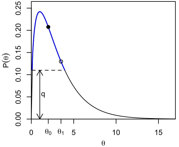
For completeness, here is one more specialization of Metropolis-Hastings that might be worth knowing about. This method reduces the need to manually tune a proposal scale, although it usually involves a rejection step (and thus "wastes" some evaluations). The procedure is for sampling a 1-dimensional PDF, meaning that it could be used within Gibbs sampling, or more generally after randomly selecting a direction in parameter space.

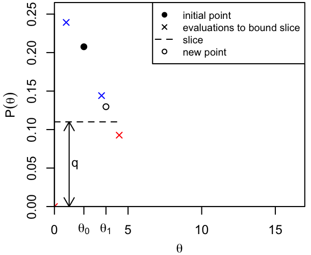
Given a starting point, $\theta_0$, we uniformly choose a probability $q\leq p(\theta_0)$. This defines a slice where $p(\theta)\geq q$, and we sample the next $\theta$ uniformly within the slice.

How to do this without actually mapping out the PDF? Here's the procedure (Neal 2003):

start with position x
evaluate p = P(x)
guess a width W
while we want samples
    draw q from Uniform(0,p)
    choose L,R: R-L=W and L<=x<=R
    while P(L) > q, set L = L - W
    while P(R) > q, set R = R + W
    loop forever
        draw y from Uniform(L,R)
        if P(y) < q,
            if y < x, set L = y
            otherwise, set R = y
        otherwise, break
    set x = y and record x

Slice sampling tends to need fewer evaluations per move than Metropolis with a poorly tuned proposal scale. On the other hand, it tends to need more evaluations per move than Metropolis with a well tuned proposal scale. Hence, slicing can be a nice option for "test chains" intended to explore the parameter space, find the high-posterior region, and roughly probe its covariance, before running a longer chain using Metropolis or some other algorithm.

Endnotes

Note 1

The output of the Markov Chain Monte Carlo, or MCMC, algorithm is a monte carlo Markov chain, or MCMC. This is less confusing than you might expect.