Notes: MCMC Diagnostics

In which we will learn about simple checks to confirm whether a Markov chain can be used for inference:

• qualitative and quantitative checks of convergence to the posterior distribution
• qualitative and quantitative checks of the autocorrelation of chains
• estimates of the number of effectively independent samples

Intuition

To be useful to us, a chain must

1. have converged to the posterior distribution
2. provide enough effectively independent samples to characterize it

Convergence means that the chain is sampling from the posterior, in contrast to the initial "burn-in" phase when the chain is finding its way to the region of high posterior density from whatever initial position it had. What would make us confident of convergence? We might ask:

• Is the chain stationary - is it (in an intuitive, average sense) staying put, as opposed to coherently moving towards a different part of parameter space?
• Do independent chains started from overdispersed positions end up in the same place?

Remember that the idea is to gather samples from throughout the posterior distribution, with the correct relative density. Getting a very long list of samples is not necessarily worth much if the random walk is taking tiny steps, such that the chain hasn't managed to move throughout the posterior. Hence the idea of effectively independent samples - if we were able to independently sample from the posterior, how many of those samples would our correlated random-walk samples be worth? Here, we can:

• Check how well the chain appears to exploring the distribution.
• Compare the autocorrelation length scale with the chain length.

There are numerical estimates that can help with this, but they are not a substitute for human visual inspection. It takes a little practice to get comfortable with making these kind of calls by inspection, but this is a situation where a trained brain does something sophisticated and difficult to reproduce mechanically.

Common misuses of/misconceptions about convergence

Convergence does not mean

• that parameters are "well constrained" by the data. If you're not satisfied with the constraints you're getting, that's a function of the data and the model, not necessarily a failing of the MCMC sampler.
• that the autocorrelation length is small. A chain can be converged and still highly correlated (though this is not desirable).
• that there are not occasional excursions beyond a locus in parameter space. If the PDF has tails, the chain will need to occasionally find its way to them; otherwise it isn't doing its job.

Convergence tests

Note that both of the checks below rely on having multiple, independently run chains, ideally started in very different parts of parameter space. This is a good idea in any case, and multiple chains that do converge can be merged (after removing the burn-in phase from each; see below) before we draw conclusions from them.

Visual inspection

Below, we can see 4 Metropolis chains (different colors) with different starting points exploring a 2-dimensional parameter space.

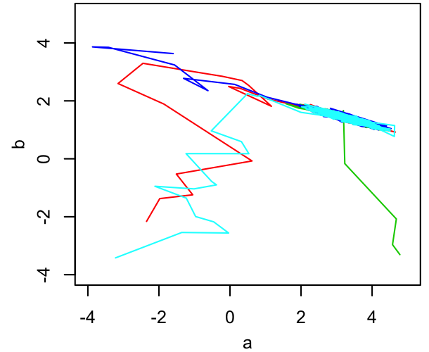
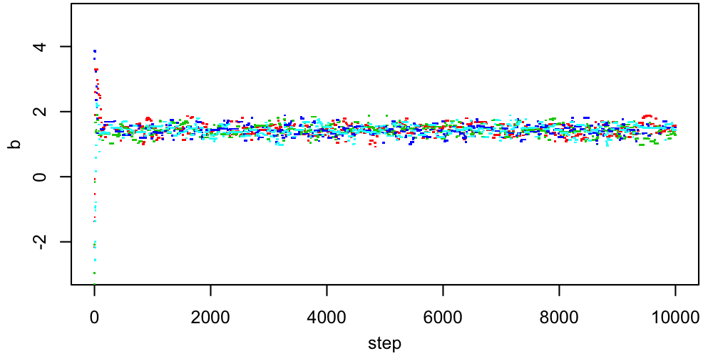
A 2D figure like this can be useful for verifying that the chains all end up in the same place, but in many dimensions it isn't really practical. More often, we would look at trace plots of each parameter, showing its value as a function of step number.

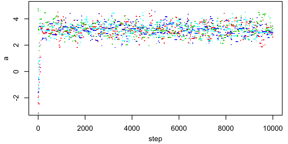
The questions to ask ourselves, based on these traces, are

• How stationary does each sequence appear?
• Do all chains look like they're sampling the same PDF?

Remember that "stationary" doesn't mean that the chain must be staying in exactly the same place. Rather, it means that one part of the chain (e.g. steps 2000-3000) should statistically resemble other parts (e.g. steps 6000-7000).

In this case, things look pretty good, apart from the early behavior corresponding to the period just after each chain is started when it's finding its way to the region where the target PDF is non-tiny. This early behavior is called burn-in, and standard practice is to remove it from the chains before computing summaries like credible intervals. In this case, we might conservatively through away the first $\sim500$ steps from each chain. After this period, the chains are mixing well (all jumbled up). This "confetti projectile vomit" appearance is what we're looking for.$^1$

Gelman-Rubin statistic

The Gelman-Rubin convergence statistic, $R$, quantitatively tests the similarity of independent chains intended to sample the same PDF. To be most meaningful, they should start from different locations and burn-in should be removed.

For a given parameter, $\theta$, the $R$ statistic compares the variance between chains with the variance within each chain. Intuitively, if the chains are random-walking in very different places, i.e. not sampling the same distribution, the variance between chains will be larger than the average of the variances within each chain. $R$ will be large in this case. If the chains have all converged to the same PDF, the between-chain variances and all the within-chain variances will be similar, and $R$ will be about 1. I practice, $R<1.1$ is often used as a requirement for convergence, but there is no magic number here.

In detail, given chains $J=1,\ldots,m$, each of length $n$,

• Let $B=\frac{n}{m-1} \sum_j \left(\bar{\theta}_j - \bar{\theta}\right)^2$, where $\bar{\theta_j}$ is the average $\theta$ for chain $j$ and $\bar{\theta}$ is the global average. This is proportional to the variance of the individual-chain averages for $\theta$.

• Let $W=\frac{1}{m}\sum_j s_j^2$, where $s_j^2$ is the estimated variance of $\theta$ within chain $j$. This is the average of the individual-chain variances for $\theta$.

• Let $V=\frac{n-1}{n}W + \frac{1}{n}B$. This is an estimate for the overall variance of $\theta$.

Finally, $R=\sqrt{\frac{V}{W}}$.

Note that this calculation can also be used to track convergence of combinations of parameters, or anything else derived from them. One useful approach is to track the convergence of the eigenvectors of the covariance of the chains (i.e. the principle components of the distribution of samples), capturing the main parameter degeneracies.

Correlation

The more correlated our chains are, the less useful information they contain per step. This is not actually a problem per se, since we could overcome it by just running the chain for longer. If we're in a situation where that would be unacceptably time consuming, the solution would be to step back and figure out a way to reduce the correlation by improving the proposal distribution. Regardless, it can be useful to have some idea how many "effectively independent" samples a chain contains.

Visual inspection

Once again, there is no substitute for the human eyeball. In these trace plots we can clearly see correlation within each chain, either repeated values or values that vary very little for many steps, before making a bigger jump. You can probably estimate by eye how many of these distinct loci each chain occupies in each parameter, post burn-in.

The degree of correlation evident in these chains is not ideal, but I would characterize it as "good enough" to work with. (However, I would probably want to run these chains for longer before calling it a day, because it seems likely that the effective number of independent samples is relatively small.)

Autocorrelation and the effective number of independent samples

The autocorrelation of a sequence, as a function of lag, $k$, can be quantified:

$\rho_k = \frac{\sum_{i=1}^{n-k}\left(\theta_{i} - \bar{\theta}\right)\left(\theta_{i+k} - \bar{\theta}\right)}{\sum_{i=1}^{n-k}\left(\theta_{i} - \bar{\theta}\right)^2} = \frac{\mathrm{Cov}_i\left(\theta_i,\theta_{i+k}\right)}{\mathrm{Var}(\theta)}$.

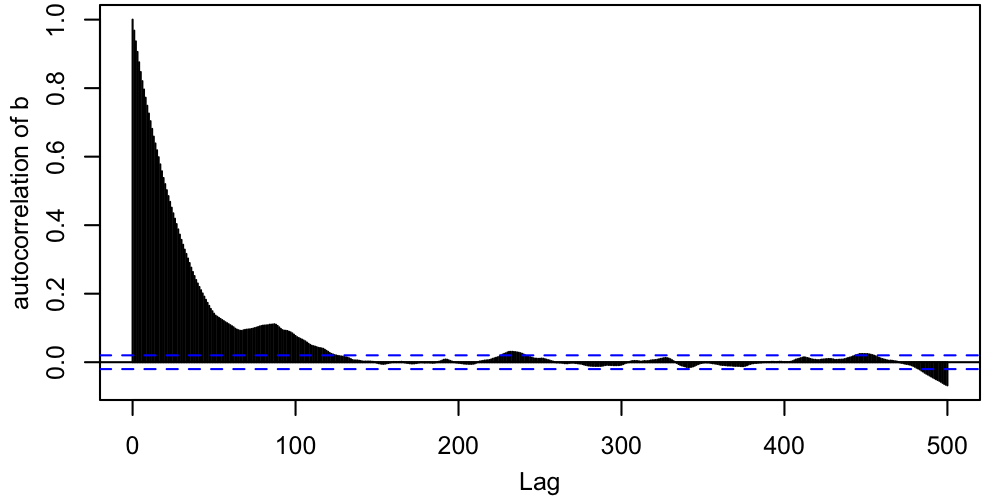
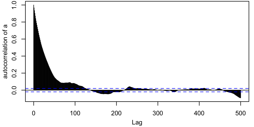
This calculation should be done after removing the burn-in phase. Generically, the autocorrelation will be large at small lags (unless the samples were actually independent rather than coming from a random walk), and eventually fall close to zero. The larger the lag one needs to get a small autocorrelation, the less informative individual samples are. Here are plots of the autocorrelation for each parameter, corresponding to one of the chains above.

The seemingly random oscillations once the autocorrelations are small roughly tell us the level of noise due to the finite chain length; the function used to produce these plots estimates this and indicates it with the dashed lines. A coherent drop as a function of lag, as both figures have at small lags, indicates a genuine autocorrelation, and the lag at which it drops to within the noise is an approximate autocorrelation length.

One could divide the chain length by this autocorrelation length to estimate the effective number of independent samples, but there is a more theoretically beautiful way.

From $m$ chains of (post burn-in) length $n$, we compute

$n_\mathrm{eff} = \frac{mn}{1+2\sum_{t=1}^\infty \hat{\rho}_t}$, with

$\hat{\rho}_t = 1 - \frac{V_t}{2V}$,

$V_t = \frac{1}{m(n-t)} \sum_{j=0}^m \sum_{i=t+1}^n (\theta_{i,j} - \theta_{i-t,j})^2$,

and $V$ (without subscript) as in the Gelman-Rubin calculation.

In practice, the sum in the denominator of $n_\mathrm{eff}$ is cut off when the estimates $\hat{\rho}_t$ become "too noisy". A practical definition of "too noisy" is, e.g., when the sum of two successive values $\hat{\rho}_t$ and $\hat{\rho}_{t+1}$ is negative.

If we wanted to, we would be reasonably justified in thinning our chains (that is selecting only a subset of samples, interspersed throughout the chain, and throwing the rest out) down to a total length of about $n_\mathrm{eff}$. However, there's no particular need to do so, unless the full chains are so long that computer memory is becoming an issue. The statistical properties of the unthinned chains are still as valid as those of the thinned chains would be (slightly more so, strictly speaking, since correlated samples still contain some new information).

Exercise: visually inspect some chains

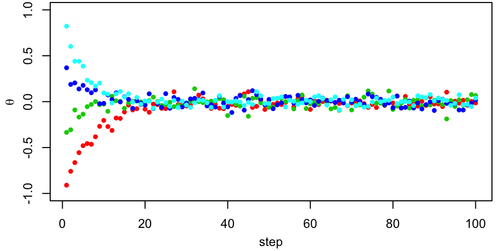
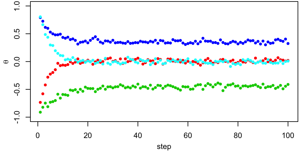
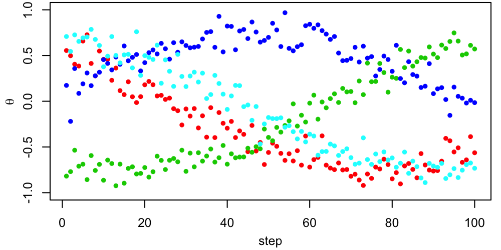
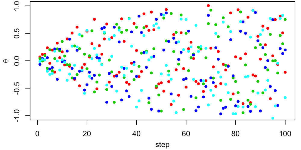
In each of the following trace plots, different colors show independent chains. For each decide by inspection whether the following are plausible claims:

1. The chains have converged.
2. The chains are highly correlated.

Answers at the end of the notebook.

How long is long enough?

How many of these "effectively independent" samples do we need?

The short and entirely unsatisfying answer is: enough that it looks good.

The longer answer is: it depends what we're going to do with the samples. If we're sampling the posterior distribution, most of the samples will (naturally) be in the region where the posterior is large. This means that it takes fewer samples to characterize the peak of the PDF well than it does to capture the tails. Statistics like means and medians converge to the correct value surprisingly quickly, 68% credible intervals take more samples (but not vastly more), 95% intervals take many more samples, and going farther into the tails generally isn't worth the effort (which is to say, we would use a different algorithmic approach if that were the goal).

More formally, the Monte Carlo error (due to the finite number of samples) of any estimate scales as $1/\sqrt{N}$, where $N$ is the number of samples, but the coefficient of this scaling depends on the estimate in question. For estimation of the PDF itself, the expected fractional error on the density scales as $\sqrt{(1-q)/qN}$, with $q$ being the true value, so that probing the tails ($q\ll 1$) does indeed become very expensive.

It takes a bit of experience to develop intuition for this, and you'll get to play around in the associated tutorial notebook.

But the bottom line is, if you're planning on showing your result graphically as a 1D posterior or 2D credible regions, the number of samples it takes to make that figure look good (smooth, i.e. lacking the noise that comes from finite sampling) will almost always be many more than it takes to robustly determine the summaries like $\theta_0\pm\Delta\theta$ that report your results quantitatively. Strange but true.

Optional extra reading

This short discussion provides some interesting context regarding how experts in the field (including the inventors of said metrics) approach the practical side of MCMC. Please do not cite these opinions as an excuse to not do visual inspection of your chains. While you are in this class, you will look at trace plots. After that, it's your funeral.

Endnotes

Note 1

An officemate of mine in grad school once declared that my thesis project must be the study of colored dots. He wasn't wrong.

Exercise answers

Top-left: converged and clearly correlated, but less so than some other examples.

Top-right: not converged, highly correlated.

Bottom-left: highly correlated; plausibly converged, though it's impossible to be certain without more steps.

Bottom-right: the least correlated; quite possibly converged, though one suspects that the data were not very constraining and we've essentially converged to a prior bounded by [-1,1]. (The starting points were chosen to be relatively close together to make this "expanding" behavior clear, in this case.)