Notes: More Modeling

In which we will

• think about complexities that often show up in astrophysical models;
• formalize what we mean by hierarchical structure in models, and how it naturally emerges;
• introduce mixture models and stochastic processes

Coping with reality

Now that you've gained some experience carrying our Bayesian inference, it's time to face the fact that real life is often more complicated than the problems we've worked so far. Some common features include:

• Heteroscedastic measurement uncertainties (i.e. different for each measurement)
• Measurement uncertainty for every measured quantity
• Correlations between measurement uncertainties, amongst different quantities and/or data points
• Intrinsic scatter (i.e. real differences that are not just due to measurement error)
• Selection effects and systematically incomplete data
• Presence of unwanted sources in the data set
• Systematic uncertainties on everything imaginable

All of these things represent something that the Universe/atmosphere/telescope/etc. has done to the signal we measure before we get our hands on it, carve it in stone, and call it data. (Insert the spicy adjective of your choice before "Universe", if you'd like.) Recalling our notes on generative models, that means that any of these effects that apply deserve to be represented in our model. In fact, all of them can in principle be handled by expanding the model appropriately, introducing nuisance parameters to encode whatever is uncertain or stochastic. The particular case of selection effects is explored more in another notebook, and all of the above issues show up somewhere (usually multiple somewheres) in the course tutorials, so you will get some practice with them. In the remainder of these notes, we will see how the commonly hierarchical structure of models naturally accomodates these complexities, and look at some of the strategies that are employed when we don't want to commit to a physically motivated model.

Hierarchical models

We introduced the concept of a hierarchical model way back in the generative models notes, and have used them several times. Let's formalize this idea, finally.

The general form for a hierarchical model goes like this:

• $p(\mathrm{data}|\theta)$ describes the measurement process (what we've been calling the sampling distribution),
• $p(\theta)$ decomposes as $p(\theta|\phi_1)\,p(\phi_1)$,
• $p(\phi_1)$ decomposes as $p(\phi_1|\phi_2)\,p(\phi_2)$,
• $\ldots$,
• $p(\phi_n)$, usually taken to be "uninformative"

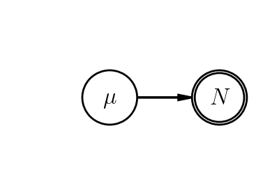
That is, a model is hierarchical if there is at least 1 non-deterministic step between the data and the farthest-upstream stochastic parameter. For example, the following, equivalent PGMs from the Bayes' Law notes are not hierarchical.

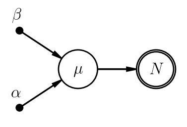Why? In both cases, our data generation consists of only (1) sampling $\mu$ from its prior, and (2) sampling $N$ from its sampling distribution, given $\mu$. Writing down fixed prior hyperparameters in the second case doesn't change the picture, and neither would inserting an arbitrary number of deterministic links between $\mu$ and $N$. In contrast, the PGM below does qualify as a hierarchy, albeit not a terribly interesting one.

We see hierarchical structures arise most naturally when we are measuring properties of multiple sources in order to learn about properties of a class of sources to which they belong. In modeling terms, the notion of a class implies that some parameter(s) describing the sources arise from a common distribution, rather than being completely unrelated to one another. In other words, even though the individual parameters describe individual objects, it's fair to apply a common prior distribution to them; the prior parameters describe the statistical properties of the source class. In statistics, the applicability of hierarchical models is related to the concept of exchangeability - meaning that, a priori, individual sources of a given class are equivalent. (This is just another way of saying the same thing - until we've made a measurement, our knowledge of any given source is just the prior PDF associated with the class it belongs to, and is the same for any of them.)

The PGM below shows an archetype of this kind of model. We have data measured for some number of $A$s (e.g. stars). The prior for their properties, $a$, depend on which class $B$ each $A$ belongs to (e.g. different galaxy types having different stellar populations). The properties of the $B$s, $b$, depend on some universal parameters $c$.

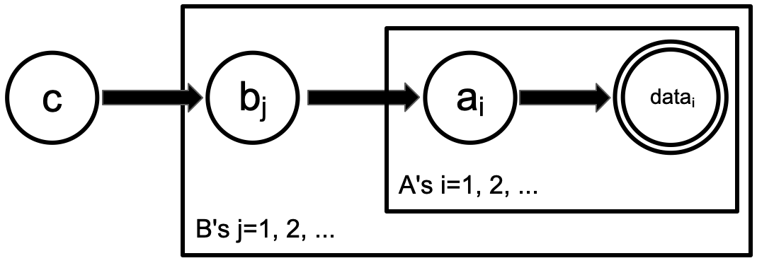Note that both of these examples would still have been "hierarchical" if we eliminated the last layer (the $c$ parameter, and the plate over $B$s in the second case).

Example: galaxy luminosity function

Let's consider a more concrete example of hierarchically modeling a class of objects as follows. Say we have measured the luminosities of a bunch of galaxies, and want to measure their luminosity function (number density as a function of luminosity).

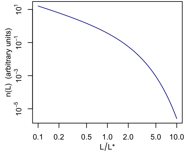
The Schechter function is a commonly used model for the luminosity function:

$n(x) = \phi^\ast x^\alpha e^{-x}; \quad x=\frac{L}{L^\ast}$.

Here's a typical curve.

For simplicity, we'll assume that we've measured every galaxy above a given luminosity in some volume. This is not very realistic, but we'll leave the issues raised by incomplete data sets for later. In essence, this assumption allows us to treat the luminosity function as being proportional to a prior PDF for the luminosities of galaxy in our data set. If we call the data for the $i$th galaxy $N_i$ and paper over the details of its relationship with luminosity, $L_i$, the PGM looks like a simple example of a hierarchical model, where the hierarchy is used to encode information about a class of objects.

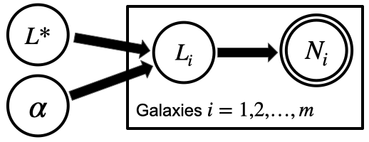(Exercise for the reader: the PGM above doesn't say anything about the $\phi^\ast$ parameter of the Schechter luminosity function, but we could relate it to the number of galaxies found, $m$.)

Mixture models

You can think of a mixture model as a complex PDF built out of simpler components. Mathematically, it has this form:

$p(x) = \sum_i f_i \, q_i(x)$,

where the coefficients $\sum_i f_i=1$, and the $q_i(x)$ are normalized.

We could interpret this as saying that $x$ belongs to one of several populations, each described by $q_i$, with probability $\pi_i$. (Equivalently, we could generate from this PDF by first choosing an $i$ based on the probabilities $\pi_i$, and then drawing $x$ from $q_i$.) Thus, one situation where this construction can be useful is when we have a data set containing multiple source classes, and aren't certain which class each source belongs to. The mixture model provides a straightforward way to marginalize over the class assignment of every source.

How does this work in practice? There are two options, either of which might be best depending on computational details. The "brute force" approach would be to literally evaluate the sum above within the posterior calculation for each source; this is numerically marginalizing over the class assignments. We might sketch a PGM like this

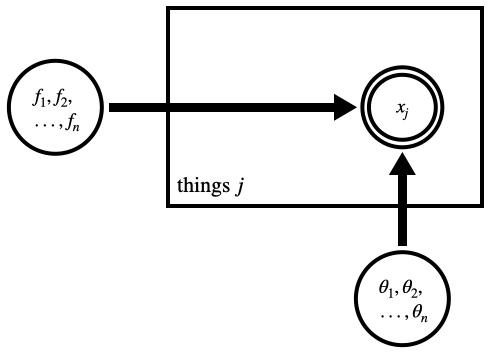corresponding to a posterior $p(f,\theta|x) \propto p(f,\theta) \prod_j \left[ \sum_{i=1}^n f_i\,q_i(x_j|\theta_i) \right]$, where $\theta_i$ parametrize the class PDFs $q_i$.

Alternatively, one can explicitly introduce a discrete parameter encoding the class of each source, e.g. $g_j \in [1,2,3,\ldots]$.

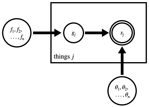The posterior would now look like $p(g,f,\theta|x) \propto p(f,\theta) \prod_j p(g_j|f) \, p(x_j|g_j,\theta) = p(f,\theta) \prod_j f_{g_j} \, q_{g_j}(x_j|\theta_{g_j})$. That is, for each source $j$, we only evaluate the sampling distribution associated with $g_j$ instead of doing the sum over possible classes. The cost of this simplification is that we now have to sample the $g$ parameters in order to marginalize over them. This isn't always a worthwhile trade-off, although it can be if (1) we want a posterior for the classification of each source for no additional effort, or (2) the model expressed in this way allows us to exploit conjugacies.

The examples above assumed that $x$ was a measured quantity being used to constrain a model, and that we had a set of sensible classes that each source could be assigned to. A different circumstance where mixture models can be useful is we simply don't have a well motivated form for some distribution, $p(y)$, appearing in our model, and want to marginalize over a more flexible range of possibilities than a single, standard PDF would provide. In this case, there is no need to associate the individual components of the mixture with anything physical, nor is there necessarily any meaning to the posterior classifications. We do, however, need to remember that such a mixture is not completely flexible, but is still constrained by the choice of PDF $q$ and the number of components. The latter, in particular, determines how much complexity $p(y)$ can have.

Let's say we have the reasonable goal of making $p(y)$ flexible enough to reflect whatever structure is in the data (presumably this is necessary for it to do its job of marginalizing over uncerainty), but no more. How would we decide on the number of mixture components? Depending on the application, we might:

1. Test how sensitive our inferences are to the number, and use the smallest number at which the results of interest "converge".
2. Do formal model comparison (e.g. via an information criterion or the evidence) to decide.
3. Explicitly marginalize over the number of components.
4. Use a number of components that we are confident is more than enough, along with a prior on the $f_i$ that favors concentrating the weight in few components rather than spreading it evenly.

Each of these, in one way or another, seeks to limit the mixture to the smallest size justified by the data.

Stochastic processes

The last application above is an example of marginalizing over an unknown PDF (i.e. not just the parameters of a known PDF, but the PDF itself). A related mathematical tool is the stochastic process. Where the PDFs we known and love describe probability distributions over numbers, a stochastic process describes a probability distribution over functions. In other words, if our function of interest is $y(x)$, a stochastic process assigns probabilities $P\left[y(x)\right]$.

Gaussian processes

The particular family of stochastic process you're most likely to encounter is the Gaussian process, for which

$P\left[y(x) | y(x_1), y(x_2), \ldots\right]$

is a Gaussian PDF whose mean and variance depend on the $x_i$ and $y(x_i)$, as well as $x$. The process is specified by a "mean function" $\mu(x)$ and a "covariance function" $C(x,x')$, or "kernel," which determines how quickly $y(x)$ can vary.

A nice feature of Gaussian processes is that all the calculations involved in the conditioning above are algebraic. In other words, if we know the value of the function at some set of $x_i$ (all the stuff conditioned on above), it's relatively easy to compute the PDF of the function value at some other $x$. Similarly, under reasonable assumptions, differentiation and integration of a Gaussian process are algebraic (citation needed).

More technically, a draw from $P[y(x^*)]$ would represent a prior prediction for the function value $y(x^*)$. But, typically, we are more interested in the posterior prediction, drawn from $P[y(x^*)\vert y_{\rm obs}(x_{\rm obs})]$, where $x_{\rm obs}$ are the locations where we know the function and $x^*$ is some other location. This posterior PDF for $y(x^*)$ is a Gaussian, whose mean and standard deviation can be computed algebraically, and which is constrained by all the previously observed $y(x)$. In its simplest form, all curves $y(x^*)\vert y_{\rm obs}(x_{\rm obs})$ with non-zero probability pass through the points $(x_{\rm obs},y_{\rm obs})$ exactly. However, the formalism for all these calculations easily extends to the case where our measurements, $y_{\rm obs}$, come from a Gaussian sampling distribution rather than being known perfectly.

Gaussian processes provide a natural way to achieve high flexibility (and uncertainty) when interpolating data, provided we're willing to make the appropriate assumptions (e.g. Gaussian measurement errors). For a given kernel, the required computations are quite efficient. Marginalization over hyperparameters such as the width of the kernel is more computationally expensive, involving the determinants of the matrices, but reasonably fast methods have been developed.

For more technical details, we recommend Rasmussen & Williams Gaussian Processes for Machine Learning.

Example: cosmography by gaussian process regression

Possibly the most widespread use of GPs in astrophysics has been to model the cosmic expansion (e.g. this article). In this context, the idea is not that the GP provides a physical model for the expansion rate, only that it provides a physics-free (though not assumption-free) alternative to making predictions from a particlar cosmological model. Typically, the formalism would then be used to decide whether GPs constrained by different data sets are compatible with one another, or whether a GP constrained from data is compatible with a particular physical model.

Given that here the GP describes the expansion rate (and/or luminosity distance, angular diameter distance, etc.) as a function of redshift, and redshifts can (spectroscopically) be measured so precisely that they may as well be fixed, this application matches well the requirements to take advantage of all the algebraic speedups available. That is, the $x_\mathrm{obs}$ where we have observations, $y_\mathrm{obs}$, to condition on can be assumed to be known without uncertainty, one of the necessary assumptions for the algebraic magic to happen. In situations like this, the use of a GP model is sometimes called Gaussian Process Regression, since it can be seen as a generalization of classical regression by (least squares).

Example: modeling unknown functions with scatter

In GP regression context, the posterior width is typically understood as our uncertainty on the function being modeled. In principle, however, GPs can also model functions that have intrinsic scatter. In the same way that a Gaussian PDF can model a mean and intrinsic variance in some quantity (e.g. the star formation rate for galaxies of a given mass), a GP would encode a mean function and intrinsic covariance (e.g. star formation rate as a function of radius for galaxies of a given mass). The latter would determine, for example, whether deparures from the mean function are coherent across a wide range in $x$ (the whole function being scaled up or down, in the extreme case), versus being less coherent (as in a particular realization wiggling back and forth across the mean many times as a function of $x$).

In this more general setting, it's easy to imagine both the $x_\mathrm{obs}$ and $y_\mathrm{obs}$ being measured with non-trivial uncertainty. The decision of what covariance kernel to use for a given application may also be challenging. In practice, problems like this are often discretized - that is, conceptually there is a GP model, but really we just fit a multidimensional Gaussian PDF to measurements at a standard set of $x_\mathrm{obs}$ (possibly using some form of interpolation to translate the original data to these $x$ values), reducing the problem to fitting a vector of mean values and a covariance matrix of a given size.

"Non-parametric" models

The last case, if we discount the GP inspiration, is an example of what is inaccurately called a "non-parametric" model. Here the idea is that we can avoid assuming a functional form for some part of our model by instead parametrizing the function in question as a series of values at given abcissa and interpolating as needed. Such a model is neither non-parametric (note the word "parametrizing" in the previous sentence); in fact, they often have a large number of parameters. Nor are they free of modeling assumptions, such as those inherent in the choice of interpolator and the number and positioning of abscissa. But, assuming those decisions can be made in a principled way, they do provide an alternative to a physically motivated model, should that be desirable.

Parting thoughts

If these notes seem a little light on concrete details compared with earlier ones, it's because we've reached the point where working through a few examples yourself is (we think) much more valuable than us pontificating about all the "advanced" models we can think of. After all, there are many ways in which models can become complex, and no single right way to handle that complexity. Similarly, while additional complexity almost invariably means more model parameters, there is no single best strategy to dealing with that computational challenge. There are a number of strategies beyond brute force MCMC that can simplify things, and there's a certain amount of artistry involved in choosing and carrying them out, as with any difficult numerical calculation. We'll see some in the tutorials here in the latter part of the course (and maybe in projects that you define). Indeed, getting you to this point, and then providing hands-on experience with realistically complex problems ("coping with reality", you might say) is one of the central goals of this course. Onward!