Notes: Missing Information, Missing Data, and Selection Effects

In which we will

• incorporate models for data selection into our toolkit
• understand when selection effects are ignorable, and when they must be accounted for

Overview

It's worth breaking down what each of the things mentioned in the title of these notes means.

Missing information just means something that we don't know. This might seem like a very silly thing to bring up so late in the course, since, from the very beginning, our models have been full of things we don't know. The simplest example of this is the true value of some quantity that we make a measurement of - we know the value of the measurement, but, unless the sampling distribution is a delta function, we'll never know the true value perfectly. These not-perfectly-known parameters tend to proliferate in hierarchical models, especially.

Missing data is just what it sounds like: data that could have or should have been measured (in some sense) but haven't been. In other words, some of those true quantities in our model aren't going to be connected to measured (and therefore constant) data values. Usually, we mean that there exist measurements of these quantities for some sources in our data set, and not others. This too may seem like a strange thing to even mention, since it doesn't obviously pose a problem for inference. Nothing prevents us from constructing a posterior distribution and/or marginalizing over those untethered parameters in the usual way. In the "worst case", they would simply be unconstrained, and their posteriors would be identical to whatever the corresponding priors dictate. (In a hierarchical model - think about the galaxy luminosity function example - those prior distributions may yet be constrained by the data that do exist, allowing us to learn something about the sources for which direct measurements do not exist.)

However, there can be issues if data are missing in such a way that the existing data set is somehow biased or not representative, yet we would like to draw unbiased inferences about a representative population. Now we have to deal with selection effects - in other words the selection process by which potentially measurable quantities are or are not measured has an effect on the data available to us. This too many seem like it doesn't pose a new problem, if we have taken the lessons from the very beginning of the course to heart, namely that the model must account for everything that determines the data. And this is true. Yet this can be tricky enough that it's worth having some notes specifically on the subject.

Here are the key messages for this lesson, of which 2-3 should not come as a surprise by now:

1. In astronomy, it's very unlikely that our data set is perfectly complete.
2. It's our job to know whether the incompleteness can be ignored for the purpose of our inference.
3. If not, we need to model it appropriately and marginalize over our ignorance.

Context

In astronomical surveys, you might hear the (historical) terms Malmquist bias and Eddington bias. These have specific meanings linked to the context where they were coined, though they are often misused to refer to selection effects more generally.

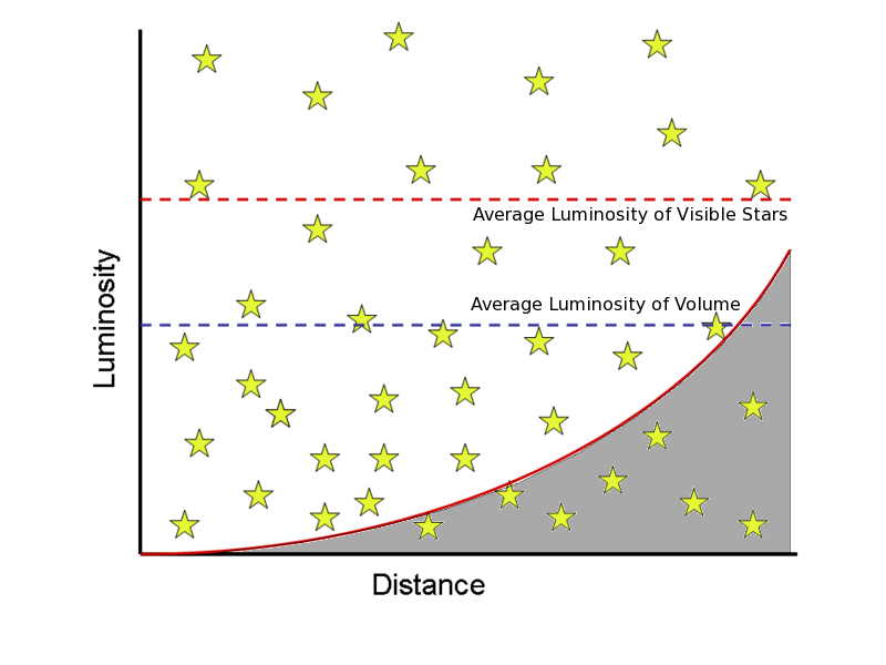
Malmquist bias refers to the fact that flux-limited surveys have an effective luminosity limit for source detection that increases with distance (redshift). Thus, the sample of measured luminosities is not representative of the whole population, where population is defined as everything above some constant luminosity. The nifty graphic below illustrates that the failure to detect sources in the shaded region leads to the mean luminosity of the available sources being larger than the mean of the complete, luminosity-limited sample.

Eddington bias refers to the impact of noise or other scatter on a measured luminosity function, the number of sources in some population as a function of $L$. (Here we need to understand the estimation procedure - measured counts would be deterministically converted to a luminosity and then a histogram of luminosities, without invoking the Bayesian machinery that you are now expert with.)

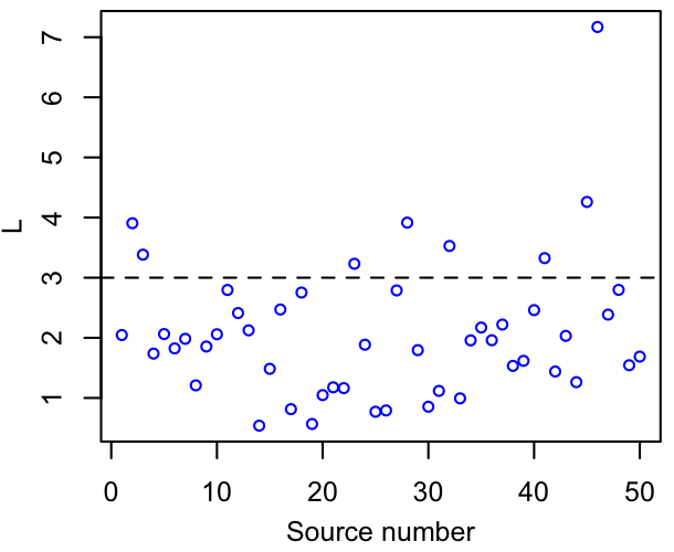
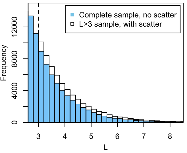
If the true $n(L)$ is steeply decreasing, the number of apparently luminous sources will be boosted relative to the truth in the presence of scatter. This happens even if the scatter itself is symmetric, simply because there are more faint sources that might be scattered up than bright sources that might scatter down. The graphics below illustrate how random, symmetric shifts - representing a sampling distribution - yield a net increase in the number of sources that exceed some threshold in luminosity. This will happen for any threshold, so long as the luminosity function is decreasing for a while below it (i.e. while there's no lack of sources to be scattered up). In the case of these simulated points, you can see by eye that the luminosity function increases rapidly to a peak at $L\sim1.5$ or $2$, and decreases rapidly thereafter.

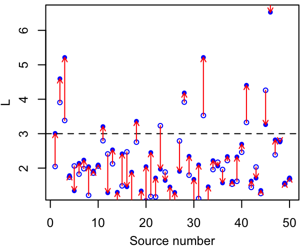All of the little shifts shown above-right lead to the bias in the estimated luminosity function below. At all luminosities above the example "detection" threshold, the scattered luminosity function exceeds the unscattered one.

These are two particular manifestations of selection effects, which we can treat in a more general framework.

In addition to these astronomical terms, there is some related terminology that you might come across in relevant statistics literature: censoring and truncation. (These are not in one-to-one correspondence with Malmquist and Eddington bias.)

Censoring means that a given data point (source) is known to exist, but a relevant measurement for it is not available. This could refer to the complete absence of a measurement, but usually this term shows up in the context of an "upper limit" placed on, e.g., the flux of a source that is independent known to exist. (Of course, the notion of an upper limit on a measurement doesn't really exist in Bayes' world, just as the "error bar" does not exist. A measurement was made, so there is a fixed constant that we can call data, and all we need to properly interpret it is the form of the sampling distribution. This naturally doesn't stop people from reporting upper limits when they fail to detect something.)

Truncation means that not only are measurements missing, but the total number of sources that should be in the data set (in the sense that they are the population we are trying to model) is unknown. In other words, the lack of a measurement means that we don't even know about a particular source's existence. Truncation is a natural feature of surveys that rely on remote sensing, which is to say all astronomical surveys, hence the fact that Malmquist and Eddington were worrying about it 100 years ago.

A concrete (albeit simplified) example

It will help to have a specific scenario in mind as we wade through the formalities. So:

LSST will include a galaxy cluster survey, finding clusters as overdensities of red galaxies (richness). The underlying cosmological signal that we care about is their number as a function of mass. Log-richness ($y$) and log-mass ($x$) are presumed to have a linear relationship with some scatter.

Complete data set

Let's start by considering the generative model for a complete data set (that is, without selection effects). It needs to include

• a mass function (number of clusters as a function of $x$), depending on cosmological parameters, $\Omega$;
• a total number of clusters in the survey volume, $N$ (also a function of $\Omega$);
• a richness-mass scaling relation (mean scaling and scatter), parametrized by $\theta$;
• true values of mass ($x$) for each of the $N$ clusters;
• true values of richness ($y$) for each cluster; and
• measured values of $x$ and $y$, $\hat{x}$ and $\hat{y}$ (we'll assume independent and known sampling distributions to keep things relatively simple).

Here is a PGM:

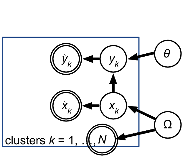Here I'm anticipating that $N$ will be a Poisson variable, whose mean is somehow computable from $\Omega$. In the absence of selection effects, i.e. with a complete data set, we know what it is, so it gets a double-circle for "data".

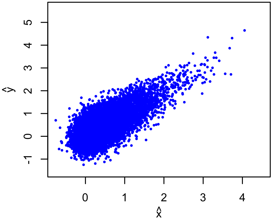
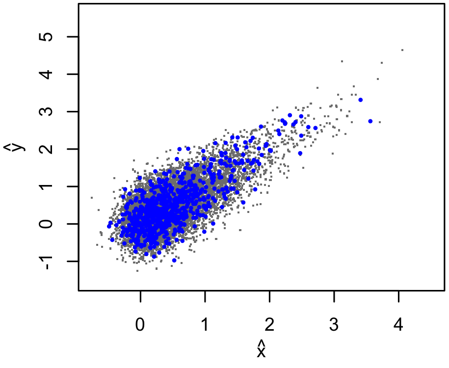
With some qualitatively reasonable parameter choices, here's a possible mock data set:

This is an inference you already know how to solve, given the modeling details. The likelihood is something like

$p(\hat{x},\hat{y},N|\Omega,\theta) = P(N|\Omega) \prod_{k=1}^{N} p(x_k|\Omega)\,p(y_k|x_k,\theta)\,p(\hat{y}_k|y_k)\,p(\hat{x}_k|x_k)$.

Truncated data set

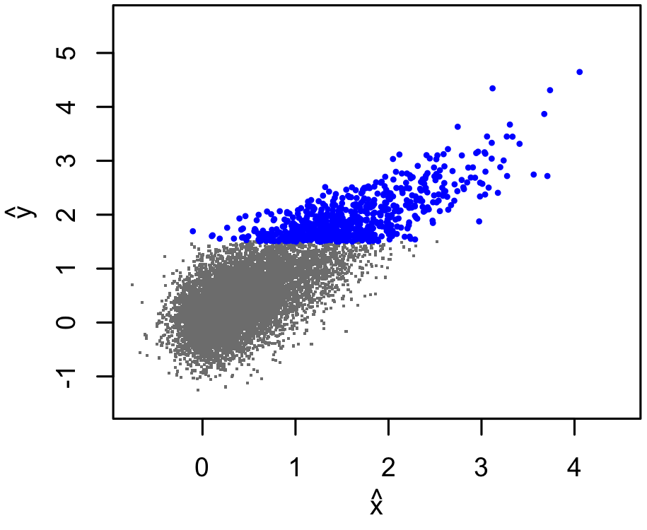
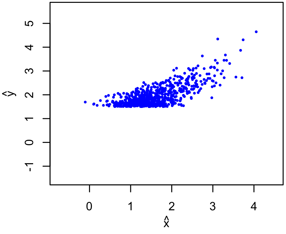
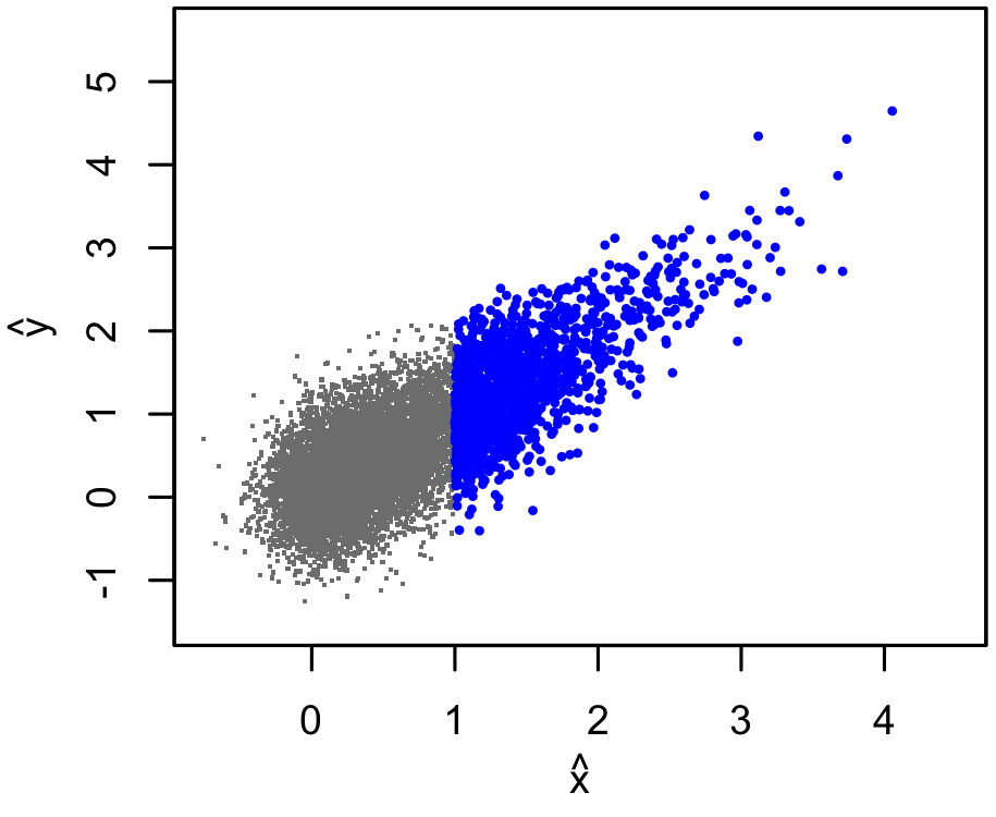
In practice, our sample will only include sources whose measured $\hat{y}$ exceeds some threshold for "detection". The total number of clusters (down to some low limiting mass) will not be known, only the number of detected clusters. So, our incomplete, truncated data set might include only the blue points below.

Needless to say, it is not safe to "simply fit a line" to the detected data, even if we only cared about the $y$-$x$ relation and not the mass function, or vice versa. Or, to be more precise, the line we get out of naively fitting the detected points is not the one that we want, which would describe the whole population.

So, how do we modify the generative model to deal with the horribly inconsiderate fact that the Universe doesn't come with a White Pages?$^1$

The answer is: we continue thinking about generating a complete data set to start with, but then apply the selection to instead model the generation of a truncated data set.

To deal with the formalities, let

• $N_\mathrm{det}$ be the number of detected clusters. It is a measurement, while $N$ is not.
• $\phi$ be any parameters that the detection probability might depend on, beyond those already present in the model.
• $I_k$ be an indicator variable (0 or 1) telling us whether the $k$th cluster in the complete generative model is detected (included in the observed data set). By definition, $\sum_{k} I_k = N_\mathrm{det}$.

Here's an expanded PGM including these new features (right).

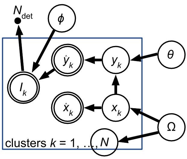What's changed?

• $N$ is no longer observed. It's now an unknown parameter!
• $\phi$ has been added.
• $\hat{y}_k$ and $\phi$ feed (possibly stochastically) into whether cluster $k$ is in the observed data ($I_k=1$) or not ($I_k=0$). $I_k$ is "measured" in the sense of being fixed by observation (it's definitely 1 for anything in the data set and 0 for anything not in the data set), as strange as that statement may sound.
• $N_{det}$ is there for completeness; it's the number of $I_k$'s that are 1.

The new likelihood can be written schematically as

$P(\hat{x},\hat{y},I,N_\mathrm{det}|x,y,\theta,\Omega,\phi,N)= {N \choose N_\mathrm{det}} \,P(\mathrm{detected}~\mathrm{clusters}) \,P(\mathrm{missing}~\mathrm{clusters})$.

Let's break this down.

The "detected clusters" term is the kind of thing we've worked with before, with the addition of the sampling distribution for $I_k=1$. Specifically,

$P(\mathrm{detected}~\mathrm{clusters}) = \prod_{k=1}^{N_\mathrm{det}} p(x_k|\Omega)\,p(y_k|x_k,\theta)\,p(\hat{y}_k|y_k)\,p(\hat{x}_k|x_k)\,p(I_k=1|\hat{y}_k,\phi)$.

The "missing clusters" term is almost the same (with $I_k=0$ instead of 1), but with the understanding that these $\hat{x}_k$ and $\hat{y}_k$ are actually unobserved, and therefore (unlike data) need to be marginalized over:

$P(\mathrm{missing}~\mathrm{clusters}) = \prod_{k=1}^{N-N_\mathrm{det}} p(x_k|\Omega)\,p(y_k|x_k,\theta)\,p(\hat{y}_k|y_k)\,p(\hat{x}_k|x_k)\,P(I_k=0|\hat{y}_k,\phi)$.

What about this binomial term, ${N \choose N_\mathrm{det}} = \frac{N!}{N_\mathrm{det}!(N-N_\mathrm{det})!}$? It's sneaky, and has to do with the statistical concept of exchangeability (a priori equivalence of data points) that we mentioned when introducing hierarchical models. We normally don't think about the fact that swapping modeled sources (within a hierarchical class) is meaningless to us when mapping generative models to inferences. Yet, for a model without selection effects, there straightforwardly are $N!$ data sets that could be generated which are perfectly equivalent apart from exchanging data points. Of course, in the case of a complete data set, this $N!$ term would be a constant, and we would normally be justified in ignoring it anyway. With our truncated data set, however, we now have to worry about the fact that our complete model constraints two non-exchangeable classes (detected and non-detected), and since the resulting binomial term includes the unknown parameter $N$ we can't simply throw it away.

It might seem like things have gotten hopeless at this point. We have a potentially enormous number of model parameters, if $N$ is large. Not only that, but the number of parameters is a variable, which means that directly sampling the posterior distribution would involve proposals to parameter spaces of different sizes, which is a level of complexity we haven't even considered before (though it can be done).

However all is not lost. First, we can simplify the "missing" term considerably due to the fact that there are no observed values to distinguish the factors in it. In particular, if we do the marginalization over $\hat{x}_k$, $\hat{y}_k$, $x_k$ and $y_k$ on paper, every term in the "missing" factor is equal, and

$P(\mathrm{missing}~\mathrm{clusters}) = \prod_{k=1}^{N-N_\mathrm{det}} \int d\hat{x}_k \, d\hat{y}_k \, dx_k\,dy_k \, p(x_k|\Omega)\,p(y_k|x_k,\theta)\,p(\hat{y}_k|y_k)\,p(\hat{x}_k|x_k)\,P(I_k=0|\hat{y}_k,\phi) = P_\mathrm{mis}^{N-N_\mathrm{det}}$,

Here $P_\mathrm{mis}$ is the lovely integral above, which now needs to be done numerically - but only once! - to marginalize over arbitrarily many of those pesky new parameters. Note that the integrand isn't trivial in the sense of automatically being unity, thanks to the presence of the $P(I_k=0|\ldots)$ term.

Second, if $P(N|\Omega)$ is Poisson, $N$ can now be marginalized out analytically to produce

$P(\hat{x},\hat{y},I,N_\mathrm{det}|x,y,\theta,\Omega,\phi)= e^{-\langle N_\mathrm{det} \rangle} \, \langle N \rangle^{N_\mathrm{det}} \,P(\mathrm{detected}~\mathrm{clusters})$.

with $\langle N \rangle$ being the mean of $P(N|\Omega)$, and $\langle N_\mathrm{det} \rangle$ being the expectation value of $N_\mathrm{det}$.

While computing these expectation values can be a pain, this leaves us with a likelihood that is a relatively simple modification of the one we started with.

Don't believe me?

There's a more intuitive, but less generally applicable, way to get to the same place. As an exercise,

• Consider modeling only the detected data. We're back to the original, simple PGM, except that $N \rightarrow N_\mathrm{det}$.
• Define a grid covering the $\hat{x}$-$\hat{y}$ plane, with cells of area $\Delta\hat{x}\Delta\hat{y}$. All our data will fall into one of these cells.
• A completely equivalent likelihood (i.e. with the same assumptions) as what we worked with above would be an independent Poisson sampling distribution for the number of detected clusters in each cell. The Poisson mean for each cell will depend on which cell it is, as well as $\Omega$, $\theta$, $\phi$ and $N$.
• Take the limit $\Delta\hat{x}\Delta\hat{y} \rightarrow 0$. (Hint: in this limit the occupation of each cell is either 0 or 1.)

Up to a constant factor of $N_\mathrm{det}!$, you'll arrive at the expression above, but explicitly marginalized over $x$ and $y$. You'll then remember the comments above about how we normally don't bother including a factor of $N_\mathrm{det}!$ in the likelihood, but technically should.

Commentary

Keep in mind that this example is not fully general. In particular, we assumed that data were independent, so that the likelihood would factor into a product over clusters, and that the prior for $N$ was Poisson. These assumptions don't always apply, but they're not uncommon approximations either.

One assumption that we made in the description and figures, but never once invoked in the derivation was that of a constant selection threshold in $\hat{y}$. In fact, we didn't really have to assume anything about $P(I_k|\ldots)$ except that it's independent of clusters other than the $k$th one. It's slightly remarkable that the final likelihood is modified only to contain the expectation values of $N$ and $N_\mathrm{det}$, and not to more directly reflect any details of the selection method.

Even so, I find it helpful to think about what information is provided by the leftmost detected point in a scatterplot like this.

Specifically, the following:

• For models that have the $x$-$y$ scaling approximately right, any detected points at the left end of the plot are going to be just above the detection limit. So their exact $\hat{y}$ values don't actually tell us much at all.
• But, the fact that there are just 3 around $x\approx0$ (say) does tell us something. It tells us that the scatter about the line, combined with the total number of sources with $x\approx0$, must be such that detecting 3, as opposed to 0 or 3000, is reasonable.
• So, as long as we see enough detected sources to have some chance at estimating the scatter, and as long as our prior $p(x)$ is reasonably accurate and not too unconstrained, we should be ok. These sources are not going to "pull" the fitted line up at the left side of the plot - in fact, they will resist such a pull because those models would predict too many detections at small $\hat{x}$.

And indeed, somewhat amazingly, it works. Granted, the need to model a hidden population places additional demands on our data, in terms of the size/quality of data set required to get a data-dominated (rather than prior-dominated) result. The need to model a hidden population also, naturally, demands that we have decent prior information about it, in the form of $p(x)$. This example is not one where we can try to marginalize over some "uninformative" or super-flexible function for $p(x)$ and expect reasonable results. (In particular, the steeply falling shape of the true $p(x)$ is not something that a typical "uninformative" hyperprior is likely to favor.) Such is the cost of doing business in a cruel and uncaring Universe.

In contrast, people have sometimes attempted to deal with selection effects simply by modifying the sampling distribution to be, e.g., a truncated Gaussian (truncated below the detection limit). This does reflect the first point above, that the lowest-$x$ sources will be barely detected. Yet the real information they provide, that they were detected at all, and in what numbers, isn't used. Consequently, the best fit for such a model (even if provided with exactly the right $p(x)$ and $N$) will still find a way to pass through those left-most detected points, rather than well below them.

Ignorability (or, when we need to care)

Unsurprisingly, fitting the data in this example without accounting for selection will wildly bias constraints on the mass function and scaling relation.

For a general problem, selection effects are ignorable if both of the following are true:

1. Priors for the interesting ($\Omega,\theta$) and selection-related ($\phi$) parameters are independent.
2. Selection is independent of (potentially) unobserved data.

Here, read "independent" in the probability sense. The second point, that selection probability may not correlate with potentially unobserved data, is often a non-starter in survey science, since whatever we're interested in usually correlates with our detection signal.

Ultimately, these conditions boil down to whether the posterior for the parameters of interest depends on selection. This makes sense; if the posterior for the parameters of interest is conditionally independent of anything selection-related, than of course we can neglect to think about selection. This is a long winded way of saying that we're welcome to simplify the problem in the sense of solving the whole thing and then simplifying the answer. There may be shortcuts when it comes to carrying out the inference, but not at the stage of setting it up conceptually.

In our example, selection depended explicitly on one of our observables, so evidently the selection is not ignorable. On the other hand, clusters that are missing because they live in a part of the sky outside of our survey are clearly not missing for reasons related to either of our observables; that particular selection effect is ignorable.

A less strict version of ignorability might be expressed as, "Does ignoring selection effects bias me at a level I care about?" Generating mock data and analyzing it lazily is the best way of answering this.

Exercise: other truncation mechanisms

Consider the following variants of the galaxy cluster example:

1. Selection is at random (not related to $\hat{x}$ or $\hat{y}$)
2. Selection is on the observed mass ($\hat{x}$)
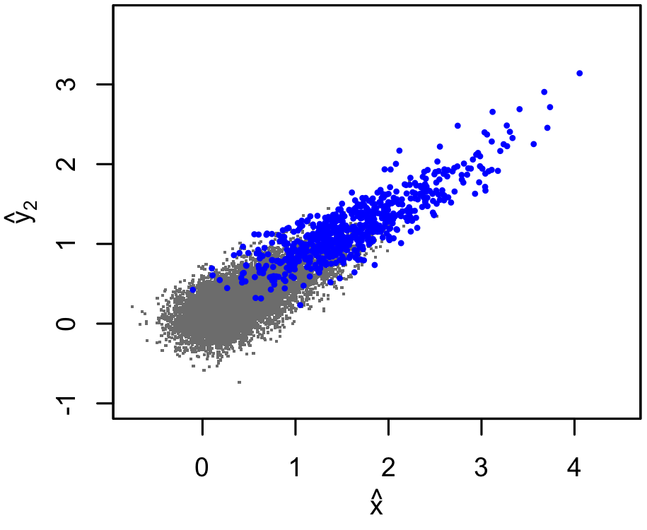
3. Selection is on $\hat{y}\rightarrow\hat{y}_1$ as before, and for detected clusters we have an additional measured observable, $y_2$, whose scaling with $x$ we want to infer

In each case, sketch the PGM and decide whether selection effects are ignorable for inference about

1. The distribution of $x$ (parametrized by $\Omega$)
2. The scaling relation parameters $\theta$ (for both $y_1$ and $y_2$, or $y_2$ alone in case 2)

If not, can you identify special cases where selection becomes ignorable?

Answers are not included in this notebook, but can be found here.

Parting words

The particular modeling complexities discussed here are, conceptually, the most challenging I've had do deal with. It was a slog to think through to the solution to the example above, it was another slog to realize that the solution is actually very simple from the right perspective, and it remains a slog to try to explain it all. Yet the basic issue of selection effects, as described above, is absolutely central to cosmology and astrophysical population studies. Unsurprisingly, therefore, this is an area where ad-hoc approaches have proliferated and remain common. So, while you may not end up using any of the results here in practice, hopefully you'll keep in mind that even in this difficult terrain there is a right way to do inference - and it follows from basic principles rather than being something that feels like it might kind of work.

Endnotes

Note 1

The "White Pages" was a book once provided by the phone company, listing the address and phone number of every customer in a given geographic area.

A book is a stack of sheets of paper, with information printed on them, generally tied or glued together along one edge.

Paper is processed trees, made into thin, uniform sheets, and once represented the primary medium by which information was transmitted and recorded.

Trees are perennial plants, generally featuring tall, structurally strong trunks and leaf-bearing branches, that periodically grow between wildfires.$^2$

The phone company (singular) was once an enterprise dedicated to providing phone service exclusively, rather than bundles of internet access and pay-per-view video.

The word "phone" once referred to a device that transmitted audio-only signals between two points via copper wire, rather than a tiny computer.

We could go on.

Note 2

Bonus fun fact: there is no such thing as a tree.