goodness

So far we have focused on the business of building a probabilistic model and using data to infer the posterior distribution of its parameters. However, model building inevitably requires making assumptions of some kind. No inference problem is really complete until we have assessed whether the data are consistent with those assumptions.

Two related but distinct questions are relevant:

Does a model explain (fit) the data well? (model evaluation)
How probable are competing models in light of the data? (model comparison)

This is a subject we'll return to in greater depth later in the course. For now, our goal is to introduce a simple method for addressing question (1) that we should, in principle, employ every single time we fit a model to data from now on. In addition, we'll explain the Bayesian approach to answering question (2), although generally doing so will require using methods that we haven't covered yet.

Throughout this discussion, as always, "model" means a complete generative model. That is, a model's definition includes the specification of prior distributions for its parameters. This is a point we often don't need to think about, but it's unavoidable when we start talking about comparing different models.

Model evaluation¶

Posterior predictions¶

A quick way to test whether our fit to the data makes sense is to look at posterior predictions, that is predictions (using the machinery of the generative model) that account for the posterior distribution of the parameters after conditioning on the data.

In the simplest case, we might look at such a posteriori predictions for our data themselves, i.e. we would compare our measurements to predictions for what we might measure (based on the sampling distribution) for parameter values drawn from the posterior distribution. If this sounds circular, it is - and that's the point! If the predictions we make from the posterior don't resemble the data that went into determining that posterior to begin with, that would be a good indication that our model assumptions have failed somewhere. (For the very simple models we've implemented so far it isn't really possible for the posterior predictions to be incompatible with the data, but for models that include physical and data collection processes this is an important test of whether our models are complete enough to really explain where the data come from.)

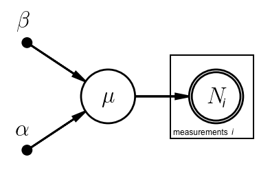
Let's do this for the final incarnation of the example from the Bayes' Law notes. Recall that we had a Poisson sampling distribution for data $N$, with the parameter of interest being the mean $\mu$, and a Gamma prior $p(\mu|\alpha,\beta)$.

At the end of the Bayes notes, we had found a posterior distribution for $\mu$ based on a whole list of measured $N$'s. To generate posterior predictions for the data, we would draw many possible values of $\mu$ from the posterior distribution, and, for each of those, draw one or more values of $N$ from the sampling distribution. In essence, we are simply using the generative model to produce mock data as we've discussed previously; however, instead of drawing model parameters from their priors, in this case we draw from the posterior distribution.

From these random realizations, we can build a histogram of predicted measurements (the posterior predictive distribution, or PPD) to compare with the histogram of actual measurements, as below.

In [2]:

data_Ns = [5, 3, 6, 5, 5, 9, 6, 8, 5, 2] # the data
# parameters of the Gamma distribution posterior at the end of the Bayes' Law notebook
alpha = 55.0
beta = 10.0

nmc = 10000 # number of posterior predictions to make
bins = np.arange(0, 18, 2);
plt.hist(st.poisson.rvs(st.gamma.rvs(alpha, scale=1.0/beta, size=nmc)), density=True, label='PPD', bins=bins);
plt.hist(data_Ns, bins=bins, density=True, histtype='step', label='data');
plt.xlabel(r'$N$', fontsize='x-large');
plt.legend(fontsize='x-large');

Qualitatively, these two distributions look basically compatible. We'll refine this below, but performing a simple comparison of data with predictions, along these lines, is a very good habit to be in.

Aside: What does this look like in math?¶

The crux of a posterior predictive test is to generate mock data from the model, with the model parameters already conditioned on the real data. If the mock data predicted by the model, when the model has already been fitted, don't resemble the data used in the fit then we have reason to suspect that the model is incomplete. In mathematical notation, if we call our real data $x$ and mock data $x'$, we want to compare $x$ with the predicted distribution of $x'$ conditioned on $x$, $p(x'|x)$.

Implicitly, above, we're conditioning on the choice of model, since this is in internal check of whether the model is working well. We are not, however, conditioning on any particular choice for the values of the parameters, $\theta$. Instead, it makes sense to allow $\theta$ to vary within its posterior distribution. Saying that the model is adequate to explain the data is more or less equivalent to saying that somewhere within the posterior for $\theta$ are values that could produce the observed data. So it makes sense that $\theta$ doesn't appear in the expression $p(x'|x)$; $\theta$ should be marginalized over, and in particular marginalized over the posterior, $p(\theta|x)$. We can write this down in math using the definition of marginalization,

$p(x'|x) = \int d\theta \, p(x',\theta|x)$,

and then factoring $p(x',\theta|x)$ using the definition of conditional probability,

$p(x'|x) = \int d\theta \, p(\theta|x) \, p(x'|\theta,x)$.

The first factor here is the posterior, and the second is the distribution of data generated by the model for given parameters. This second term is conditionally independent of $x$; after all, we could produce mock data given parameter values from a generative model even if no real data had been collected. So we can finally simplify to

$p(x'|x) = \int d\theta \, p(\theta|x) \, p(x'|\theta)$.

The above expresses in an equation the procedure we described above: we generate mock data from the model while marginalizing the model parameters over the posterior distribution, which was found by analyzing the real data.

Notice that the "$|x$" is just carried along throughout the above manipulations. This conditioning is what makes the test a posterior check. Had we not done so, the equation

$p(x') = \int d\theta \, p(\theta) \, p(x'|\theta)$

would describe generating mock data from the prior distribution of $\theta$. Seeing whether this distribution is compatible with the real data might be interesting, but it's a less stringent test than the one using $p(x'|x)$. (Note that none of the quantities above is the evidence, despite a superficial resemblance. Real data are constants, so the evidence, $p(x)$, is a number; in contrast, mock data, $x'$, are random variables, and so $p(x')$ and $p(x'|x)$ are both PDFs defined over the domain of $x'$.)

Test statistics¶

The data and PPD above look similar but not quite the same. Then again, with only 10 measurements in our data set, we'd expect a certain amount of noisiness in a histogram of our data that doesn't exist in the PPD if we've generated a large number of mock observations. This suggests that, perhaps, a more sensible comparison would be between a single number summarizing our data set with the same number computed from mock data sets of the same size. That single number is called a test statistic: something that can be computed from real or mock data for the purposes of comparison.

Given that we're trying to measure a mean, it seems reasonable to choose the mean of the data as our test statistic:

$T(\{N_i\}) = \bar{N}$.

Let's see how $\hat{T}$, the test statistic computed on our real data, compares with the distribution of $T$ predicted for data sets of equal size.

In [3]:

T = np.mean # function to compute the test statistic
T_data = T(data_Ns)

nmc = 10000 # number of posterior predictions to make
T_pred = [T(st.poisson.rvs(st.gamma.rvs(alpha, scale=1.0/beta), size=len(data_Ns))) for i in range(nmc)]

plt.hist(T_pred, density=True, label='PPD', bins=20);
plt.axvline(T_data, label='data', color='C1');
plt.xlabel(r'$T$', fontsize='x-large');
plt.legend(fontsize='x-large');

Now that we have just one number to compare between the real data and the PPD, it's straightforward to say that yes, $\hat{T}$ is compatible with the distribution $p(T|\mathrm{data})$. If we wanted to, we could quantify this in terms of the fraction of predictions for $T$ that were more extreme than $\hat{T}$, $P(T>\hat{T})$. If $P(T>\hat{T})$ were sufficiently extreme, say $<0.01$ or $>0.99$, we might be tempted to look for an alternative model to explain the data.

Note that the test statistic was something that we had to choose, even if the choice in this simple case was fairly straightforward. In general, there isn't a correct choice; it depends on what we're trying to accomplish. For example, if we don't really expect any model to explain the data in detail, but just want something that describes a particular feature of it, then we would choose $T$ to reflect that feature. More generically, the maxmimum log-likelihood achievable for the data under the model in question is common choice, as we'll see later.

Model comparison using Bayesian evidence¶

As you'll doubtless recall from the Bayes' Law notes, the evidence is the normalizing constant of the posterior distribution, $P(\mathrm{data}|\mathrm{model})$, as in

$P(\mathrm{params}|\mathrm{data},\mathrm{model}) = \frac{P(\mathrm{params}|\mathrm{model})\,P(\mathrm{data}|\mathrm{params},\mathrm{model})}{P(\mathrm{data}|\mathrm{model})}$.

To condense the notation somewhat, let $H$ stand for a choice of model, including the prior distributions of its parameters, $\theta$ stand for those parameters, and $D$ stand for the data. Then the form of Bayes' Law above, where we explicitly show that inferences about the parameters depend on the choice of model, is written

$P(\theta|D,H) = \frac{P(\theta|H)\,P(D|\theta,H)}{P(D|H)}$,

and the evidence is $P(D|H) = \int d\theta P(\theta|H)\,P(D|\theta,H)$.

When we're only interested in inferring the parameters $\theta$ for a chosen $H$, we generally don't need to explicitly compute the evidence. It's utility is in applying Bayes' Law at the level of the model itself. Imagine we have a set of possible models that we're considering, $\Omega$; then a Bayesian inference of the probability of model $H$ takes the form

$P(H|D,\Omega)=\frac{P(D|H,\Omega)P(H|\Omega)}{P(D|\Omega)}$.

Here

$P(H)$ is a prior probability distribution over models in $\Omega$;
$P(D|H)$ is the evidence for model $H$, which now takes on the role of the sampling distribution; and
$P(D|\Omega)$ is a new normalizing factor (meta-evidence!), which we will firmly sweep under the rug. (Unless, of course, we wanted to compare the likelihood of one set of models with another, something I have not seen in practice.)

Since the space of possible models is not continuous as such, it makes little sense to think about credible intervals in this context. We could, however, think about comparing the ratio of posterior probabilities of two models,

$\frac{P(H_2|D)}{P(H_1|D)}=\frac{P(D|H_2)\,P(H_2)}{P(D|H_1)\,P(H_1)}$,

to decide which provides a better explanation of the data.

In the example problem from the Bayes' Law notes (and above), we found an analytic form for the evidence. Usually such a convenient solution will not be available, so we won't return to the evidence until after introducing a number of numerical methods that we use to characterize posterior distributions in more general cases. However, as an illustration, let's work out a slightly contrived model comparison using the evidence in the simple example.

In fact, to simplify as much as possible, consider the case where we have a single measurement, $N=5$. We found in that case that the evidence is

$P(N) = \frac{\beta^\alpha}{\Gamma(\alpha)N!} \frac{\Gamma(\alpha+N)}{(\beta+1)^{\alpha+N}}$.

Recall that $\alpha$ and $\beta$ are the hyperparameters of the prior for $\mu$, our sole model parameter.

In order to keep everything conjugate (and therefore analytic), let's consider comparing two models that have the same Poisson sampling distribution but different prior distributions for $\mu$. This might seem like too trivial a change to qualify as creating a "different" model, but in general one can imagine that one physical model might imply a strong prior on some parameter, while a competing model might not. In any case, it will do for an illustration.

So, imagine $H_1$ has the uniform prior we used previously, encoded by hyperparameters

$H_1$: $\alpha=1$, $\beta=0.0001$,

while $H_2$ has a prior for $\mu$ that is, for some reason, sharply peaked at 10

$H_2$: $\alpha=400$, $\beta=40$.

The cell below visualizes these priors for $\mu$.

In [4]:

plt.rcParams['figure.figsize'] = (6.0, 4.0)
mu = np.linspace(0.1, 15.0, 150)
plt.plot(mu, st.gamma.pdf(mu, 1.0, scale=1.0/0.0001), '-', label=r'$p(\mu|H_1)$');
plt.plot(mu, st.gamma.pdf(mu, 400.0, scale=1.0/40.0), '-', label=r'$p(\mu|H_2)$');
plt.xlabel(r'$\mu$', fontsize='x-large');
plt.legend(fontsize='x-large');

How do the (log) evidences for these models compare?

In [5]:

def log_factorial(x): # is this seriously not in numpy/scipy?
    return loggamma(x + 1.0)

def log_evidence(alpha, beta, N):
    return alpha*np.log(beta) - loggamma(alpha) - log_factorial(N) + loggamma(alpha+N) - (alpha+N)*np.log(beta+1.0)

In [6]:

print('log-evidence for H1:', log_evidence(1.0, 0.0001, 5))
print('log-evidence for H2:', log_evidence(400.0, 40.0, 5))
print('Ratio of evidences, H2/H1:', np.exp(log_evidence(400.0, 40.0, 5)-log_evidence(1.0, 0.0001, 5)))

log-evidence for H1: -9.210940341978183
log-evidence for H2: -3.2501676095109815
Ratio of evidences, H2/H1: 387.90975891921175

Keep in mind that this ratio of evidences is not the same as the ratio of posteriors for the models, unless we for some reason gave them equal prior probability. Since this is a completely fictional example, we won't think too hard about priors, but in general they deserve careful thought. So, model priors aside, where does this preference for $H_2$ come from? To understand, let's have a look at the parameter priors in each model in comparison to the common likelihood for our measurement of $N=5$. The plots below does this with linear and log axes.

In [7]:

plt.rcParams['figure.figsize'] = (12.0, 4.0)
fig, ax = plt.subplots(1,2)
ax[0].plot(mu, st.gamma.pdf(mu, 1.0, scale=1.0/0.0001), '-', label=r'$p(\mu|H_1)$');
ax[0].plot(mu, st.gamma.pdf(mu, 400.0, scale=1.0/40.0), '-', label=r'$p(\mu|H_2)$');
ax[0].plot(mu, st.poisson.pmf(5, mu), label='likelihood');
ax[0].set_xlabel(r'$\mu$', fontsize='x-large');
ax[0].legend(fontsize='x-large');
ax[1].semilogy(mu, st.gamma.pdf(mu, 1.0, scale=1.0/0.0001), '-', label=r'$p(\mu|H_1)$');
ax[1].semilogy(mu, st.gamma.pdf(mu, 400.0, scale=1.0/40.0), '-', label=r'$p(\mu|H_2)$');
ax[1].plot(mu, st.poisson.pmf(5, mu), label='likelihood');
ax[1].set_xlabel(r'$\mu$', fontsize='x-large');
ax[1].set_ylim(1e-7, 1e5);
ax[1].legend(fontsize='x-large');

The key feature that comes over here is that the $H_2$ prior is far more sharply peaked than the $H_1$ prior. In other words, model 2 is a priori far more predictive about $\mu$ than model 1. Model 1, in contrast, is fine with any non-negative value of $\mu$, and thus the prior probability for any of them is tiny.

The evidence, by virtue of weighting the likelihood by the prior in its integration, explicitly rewards models that are more predictive... provided they can explain the data. In this case, even though that sharp peak in the $H_2$ prior doesn't align with the peak of the likelihood, the $H_2$ is still orders of magnitude larger than the $H_1$ prior in a range where the likelihood is modestly large. Numerically, this translates to a larger evidence by a factor of a few hundred. A similarly tight prior centered a little closer to $\mu=5$ would be preferred by a factor of 1000 or more.

This penalty for wide parameter priors is a manifestation of Occam's razor, the notion that a model with greater flexibility should have to justify itself by doing a much better job at explaining the data, given that generically grater flexibility should be expected to improve the fit whether or not it's meaningful. You can imagine the extreme version of the example above, in which $H_2$ makes the a priori prediction that $\mu=5$ exactly, and we have made enough measurements that the likelihood peaks very sharply at the same spot. In that case, we would probably be pretty impressed by the foresight of whoever came up with model 2 (having not seen the data), and it might make sense to conclude that, indeed, model 2 is much more probable given the data than model 1.

Lest you leave with the impression that the evidence is only a measure of the prior width, keep in mind that this is a somewhat contrived example that illustrates how silly it is to chose absurdly wide priors, as in $H_1$. A more interesting scenario is when both models are somewhat constrained a priori, and the difference in evidence more clearly depends on which one makes predictions that are closer to the data. Let's see how this works by introducing

$H_3$: $\alpha=16$, $\beta=4$.

In [8]:

plt.rcParams['figure.figsize'] = (6.0, 4.0)
plt.plot(mu, st.gamma.pdf(mu, 400.0, scale=1.0/40.0), '-', label=r'$p(\mu|H_2)$');
plt.plot(mu, st.gamma.pdf(mu, 16.0, scale=1.0/4.0), '-', label=r'$p(\mu|H_3)$');
plt.plot(mu, st.poisson.pmf(5, mu), label='likelihood');
plt.xlabel(r'$\mu$', fontsize='x-large');
plt.legend(fontsize='x-large');

Here is how the evidence compares with $H_2$:

In [9]:

print('log-evidence for H2:', log_evidence(400.0, 40.0, 5))
print('log-evidence for H3:', log_evidence(16.0, 4.0, 5))
print('Ratio of evidences, H3/H2:', np.exp(log_evidence(16.0, 4.0, 5) - log_evidence(400.0, 40.0, 5)))

log-evidence for H2: -3.2501676095109815
log-evidence for H3: -1.9686330490673072
Ratio of evidences, H3/H2: 3.6021632236091596

Despite having a prior about twice as wide (in standard deviation), $H_3$ ends up being modestly favored because it is more compatible with the data. Both models are still reasonable - consider how wide the the likelihood curve is above - but the evidence would clearly nudge us towards prefering $H_3$ to $H_2$.

Concluding remarks¶

This particular set of notes contains a mix of the immediately useful, and things we will not really take advantage of until later on. This is because the utility of the evidence, and test statistics to a lesser extent, is limited while we are still working with very simple inference problems. Before we see these ideas in action, we will need to cover the numerical techniques that make it possible to solve more complex inference problems than those we have seen so far.