Notes: Credible Intervals and Regions

Containing:

• An explanation of and opinions about various conventions for summarizing posterior PDFs

Summarizing 1D posterior distributions

The posterior distribution is The Answer to an inference problem, but a PDF over potentially many dimensions is a cumbersome beast. Often, what we want to do is summarize the constraints on one or more parameters with a statement like $\theta = \theta_0 \pm \Delta\theta$ or $\theta = \theta_0{}_{-\Delta\theta_m}^{+\Delta\theta_p}$. These should be interpreted as statements about the marginal posterior of $\theta$, namely that $\theta$ is in the given credible interval (CI) with some specified probability. To be explicit, if $\theta$ is the parameter of immediate interest, and $\phi$ are all the other parameters, the marginal posterior distribution of $\theta$ is

$p(\theta|\mathrm{data}) = \int d\phi \, p(\theta,\phi|\mathrm{data})$,

and a credible interval for $\theta$ containing probability $q$ satisfies

$\int_\mathrm{CI} d\theta \, p(\theta|\mathrm{data}) = q$.

Note that credible intervals/regions are technically different from the confidence intervals/regions that appear in non-Bayesian statistics, which we'll touch on in later notes. Unfortunately, in practice, the terms are often used interchangeably. Apologies in advance if that happens in this course.

Saying that a 68% CI contains a probability of 0.68 doesn't uniquely tell us how to define the interval, nor what "best" value we should report as $\theta_0$, and in practice there are multiple conventions. Let's look at a few of them.

Aside: significant digits

The convention that I learned back when dinosaurs roamed is that we report results to the leading digit of the uncertainty, unless that digit is a 1, in which case we go one further. For example,

$3.14159 \pm 0.27182 \rightarrow 3.1 \pm 0.3$

but

$3.14159 \pm 0.16180 \rightarrow 3.14 \pm 0.16$.

This is a pretty good default rule. In real life, you might add more "precision" to satisfy the convention used for a particular measurement, or just to make the entries in a table uniform.

Most probable value and interval

This is also sometimes known as "highest posterior density" (HPD).

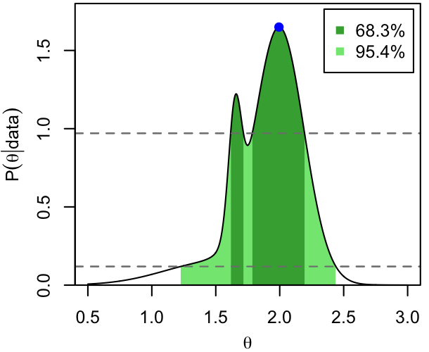
Quite simply, this convention would report as $\theta_0$ the mode of the marginal posterior. The credible interval is the (possibly multiply connected, i.e. consisting of multiple, disjoint intervals) interval of largest posterior density that contains the specified probability. Consequently, it is also the smallest possible interval containing the target probability.

To help visualize this, the following is one method for determining the HPD interval(s):

• Choose some threshold value of probability density to begin with.
• Integrate the PDF within the interval(s) where it exceeds the threshold.
• Repeat the last step, adjusting the threshold density until the integral (the probability enclosed by the intervals) is what we want it to be.

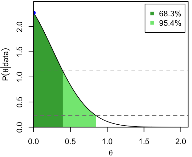
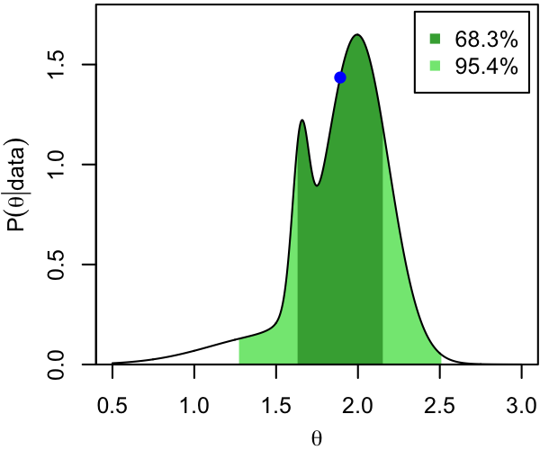
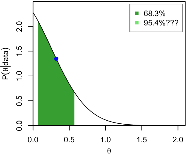
The modes (blue dots) and 68.3% and 95.4% CI's are shown below for 3 (unrelated) PDFs that we'll use as exemplars throughout these notes.

1. A standard (mean 0, variance 1) normal distribution, about as simple as they come.
2. An asymmetric distribution with multiple modes.
3. A very asymmetric distribution, peaking at the edge of the allowed region for its parameter (you might imagine this as providing an "upper limit" for a mass or flux, which cannot be negative by definition).

Dark and light shading show the extent of the two intervals, while the horizontal, dashed lines show the corresponding thresholds in probability density. That is, per the definition and the procedure above, the 68.3% CI consists of all those values of $\theta$ for which $p(\theta|\mathrm{data})$ exceeds the higher dashed line.

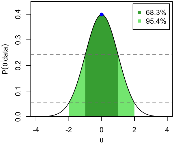
Advantages: I would argue that this definition is by far the most intuitive. The nominal value we report is actually the "best" in the sense of most probable given the data, and similarly the interval contains the most probable values. Faced with the statement $\theta = \theta_0 \pm \Delta\theta$, what else would one possibly think?

Similarly, the mode/HPD convention in the right-hand case clearly represents the fact that the posterior is peaked at zero (we would write $\theta=0^{+\Delta \theta}_{-0}$), which the other approaches discussed below would not do.

Finally, this method straightforwardly generalizes to multidimensional credible regions (below), unlike the next option.

Disadvantages: When the CI is multiply connected (the second case, but highly unusual in my limited experience), it's more annoying to describe. Also, when we use Monte Carlo methods to characterize the posterior, we will need to use kernel density estimation (a fancy way to say "smoothing a histogram") to get a smooth function from a finite number of samples; the precise value of the mode and CI limits can be rather sensitive to these details, though generally not at a level that matters (see Significant Digits, above). This means that a human needs to at least look at the distribution to verify that the results are ok (horrors!). I know of exactly one Python package that computes this style of CI correctly, including the multiply connected case, and it's the one I wrote (so, you know, tech support is questionable).

Median value and symmetric interval in probability (percentile) space

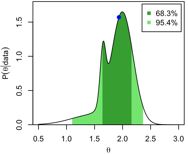
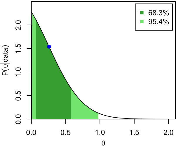
In this convention, $\theta_0$ is the median of the marginal posterior, and the endpoints of the CI containing probability $q$ are the quantiles corresponding to probabilities $(1-q)/2$ and $(1+q)/2$. So, for example, the 68.3% CI spans the quantiles of 0.1585 and 0.8415. Note that the CI is not necessarily symmetric about $\theta_0$. Here is how it looks for the same 3 PDFs.

Advantages: Straightforward to automatically compute from monte carlo samples or evaluations on a grid without human intervention or thought. This is the method I would recommend when the result being reported is not the result of the work, and the more eyes-on method above isn't feasible (e.g. when you need to plot many measurements in a figure). For a unimodal and symmetric PDF like the first example, these CI's are identical to those from the HPD method, so the percentile method is easily defensible when the PDF in question approximately satisfies those requirements.

Disadvantages: If the PDF is not actually unimodal and symmetric, the nominal value and CI reported are not the most probable! In cases resembling the second and third examples, the CI can be... non-intuitive. One wouldn't guess from the median and percentile-based CI that the posterior is sharply peaked at zero in the righ-hand plot above, for example. This method also lacks an obvious multidimensional analog.

Mean value and symmetric interval

Here we would (if we were silly) report the mean of the PDF as $\theta_0$, and build a CI by extending symmetrically (in $\theta$) in both directions until we contain the right probability.

Advantages: None that I know of. It will produce identical estimates to the other methods above for perfectly symmetric and unimodal distributions like the left-hand example, but it's not really any easier to compute than the second method.

Disadvantages: Even odder behavior for asymmetric/multimodal distributions than the last method. If the PDF has a sharp cutoff (e.g. due to the prior going to zero), the CI can easily extend into this forbidden region. I don't even want to contemplate how one might extend this to multiple dimensions.

Needless to say, this option is not recommended, but you might see it occasionally.

Other conventions

For completeness, two more methods are worth mentioning. Each of these is only valid (in the sense of even delivering the advertised contained probability) in certain limits, namely as (and if) the central limit theorem makes the posterior Gaussian.

• CI's defined from differences in the log-likelihood or log-posterior, following the Maximum Likelihood tradition. This can be quite accurate in situations that satisfy the central limit theorem, even if the posterior isn't quite Gaussian, but doesn't present any particular advantages, computationally speaking.
• Reporting the mean and standard deviation of the PDF. Please don't do this. It's hardly any computationally easier than finding the percentiles of a distribution, but only valid (in the sense of corresponding to known enclosed probability) for a Gaussian.

Summarizing multi-dimensional posterior distributions

It's also common to visualize 2D marginalized posteriors (that is, marginalized over all but 2 parameters),

$p(\theta_1,\theta_2|\mathrm{data}) = \int d\phi \, p(\theta_1,\theta_2,\phi|\mathrm{data})$.

Most often, we don't try to show the PDF itself or report numbers inline, but just plot the contours delineating the 2-dimensional credible region(s). These are defined analogously to the 1D case as regions (CRs) that contain a specified amount of probability of the 2D marginalized posterior. As far as I know, the only convention in wide use for how to uniquely define the regions is the "most probable" one. (You might occasionally see the analog of the "mean and standard deviation" method, in which the covariance matrix translates to a 2D ellipse, but this is not suddenly a better idea in multiple dimensions than it is in 1D.)

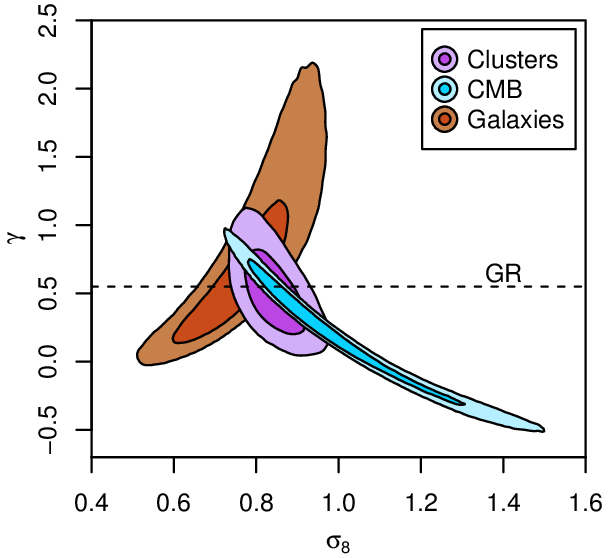
One reason to look at 2D posteriors is that they reveal degeneracies between parameters, i.e. loci in parameter space in which the posterior is constant or slowly changing. In the example below, you can see that the posterior for each analysis shown has a degeneracy between the parameters $\sigma_8$ and $\gamma$, but the direction and strength of these degeneracies (roughly, the orientation of the contours and how drawn out they are) vary. Here we can see that jointly analyzing all 3 data sets could result in much tighter constraints, since the area where the posteriors are simultaneously large is relatively small, something that might not be obvious from the 1D posterior distributions alone.

Generally, a 1D CI will have a smaller extent in a given parameter than the 2D CR for the same contained probability. This is not a bug, but follows from the fact that the 1D marginalized posterior is integrated over an additional degree of freedom compared with the 2D one, which can result in the 1D PDF being more sharply peaked. In the case above, if we looked at only the 1D posteriors, we might be led to believe that the "Galaxies" and "CMB" posteriors were inconsistent with each other, while in 2D we can see that they overlap nicely.

When there are interesting or relevant degeneracies, as in this case, best practice is to show them with a plot like the one above. The 1D CIs that we might put in a table could still be as described above, regardless of the degeneracy. Rarely, it might make sense to report a CI for a combination of parameters that is well constrained by the data, e.g. corresponding to the short axis of one of the contours above. But, as this example shows, the relevant axis is rarely the same for different types of data that might constrain a model, and may not even be the same for different data sets of the same type. So this approach is of limited utility. For example, the short axis of the Galaxies constraints is approximately aligned with the long axis of the CMB constraints above. If we reported 1D CIs corresponding to that direction in parameter space, it would seem that Galaxies were much more constraining than the CMB (or vice versa), but this hardly provides a clear picture of how the two data sets complement one another, as the 2D plot does.

Naturally, features like degeneracies can exist in more than 2 dimensions, but there isn't a widely used method for visualizing CR's in more than 2D. You may encounter color being used to show the most probable value of a third parameter at different points in the $\theta_1$-$\theta_2$ plane, but that's about it.

What's so special about 68.3% and 95.4%?

These numbers are a legacy of the centrality of the Gaussian distribution in statistics. You might recognize them as approximately the integral of a Gaussian from $-1\sigma$ to $+1\sigma$ (68.3%) and $-2\sigma$ to $+2\sigma$ (95.4%), where $\sigma$ is the standard deviation. Consequently, they are often referred to as "$1\sigma$ confidence" and "$2\sigma$ confidence". (This is another bit of terminology that we will almost certainly slip into, despite it not being technically meaningful.)

Regardless of the origin, these are conventional probability levels in our field. It's not so bad. Roughly speaking, you can just think of 68.3% as $2/3$ and 95.4% as $19/20$; conversely, there's a 1 in 3 chance that the 68.3% CR doesn't include the truth, but only a 1 in 20 chance that the 95.4% CR does not. Please note, though, that the difference between 95.0% and 95.4% is not necessarily quantitatively trivial; we aren't just being pedantic by including the third significant digit here.

Most often, you will see 68.3% and 95.4% CR's shown in 2D contour plots, and 68.3% CI's reported in text (though often 95.4% is used when quoting a limit). In practice, we don't often see higher probability values because (a) we don't normally care, and (b) robustly determining the CIs/CRs becomes increasingly computationally expensive for higher probabilities.

If you ever forget these magical percentages, or need to know them to higher precision, or need to find the probability associated with more than $2\sigma$, the definite integral of a Gaussian is simple to compute using the normal CDF:

import scipy.stats as st
def probLevel(Nsigma):
    return st.norm.cdf(Nsigma) - st.norm.cdf(-Nsigma)

However, this can be done even more simply using the chisquare distribution. By definition, the $\chi^2(\nu=1)$ distribution describes the square of a standard normal random variable. Since $P(-N<Z<N) = P(Z^2<N^2)$ must be true for any real-valued $Z$, we could equivalently write the function above with a single call:

def probLevel(Nsigma):
    return st.chi2.cdf(Nsigma**2, 1)