In which we will
Now that you've gained some experience carrying our Bayesian inference, it's time to face the fact that real life is often much more complicated than the problems we've worked so far. (The original title of these notes, years ago, was "Coping with Reality".)
In any case, real data sets tend to be complicated. Some common features:
All of these things represent something that the Universe/atmosphere/telescope/etc. has done to the signal we measure before we get our hands on it, carve it in stone, and call it data. (Insert the spicy adjective of your choice before "Universe", if you'd like.) Recalling our notes on generative models, that means that any of these effects that apply deserve to be represented in our model. Very often, this involves introducing additional nuisance parameters and/or expanding the model such that it has a hierarchical structure. We've seen both of these features before, in fact, but it's time to give them a name and see how enabling they really are.
A nuisance parameter is any model parameter that we are not particularly interested in learning about, at the end of the day. This is an entirely subjective label - nuisance parameters are not formally or functionally treated any differently from other parameters. We're coming back to them now because adding nuisance parameters to a model provides a way to explicitly account for and marginalize over systematic uncertainties. This can be as simple as assigning a prior distribution to some quantity that would otherwise remain fixed, or it can involve a more explicit expansion of the model. Nuisance parameters often represent latent variables - things that are logically or physically part of a model, but which cannot be directly measured.
Recall our simple measurement of a source's flux based on a number of detected counts from way back in the Bayes' Law notes. Let's explicitly include the constant conversion between flux and counts, so that our model might be described by
The form of the prior on $F$ isn't critical for our purposes here, so we'll stick with the Gamma distribution. The corresponding PGM looks like this:
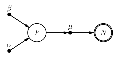
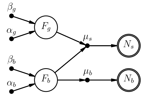
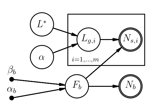
Now let's expand the model to account for the fact that our measurement actually includes counts from both the source (a galaxy, say) and some background. Being good astronomers, we also remembered to take a second measurement of a source-free (background-only) patch of sky.
With subscripts $b$ for background, $g$ for galaxy, $s$ for the science observation that includes both, our model might be
We'd probably regard $F_b$ and $\mu_b$ as nuisance parameters here - we need to account for our uncertainty in $F_b$, but measuring it isn't the point of the analysis.
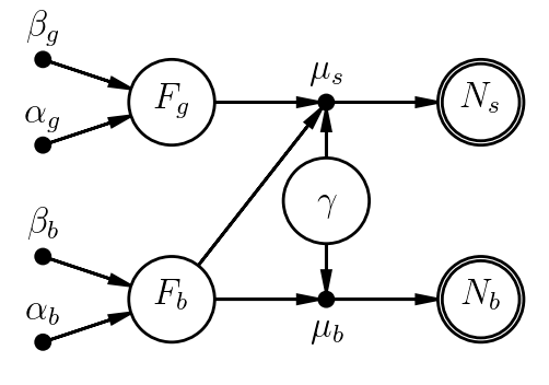
More interestingly, suppose we want to marginalize over systematic uncertainty in the instrument gain, assuming it's the same for both observations. Maybe the instrument team told us it was known to $\sim5\%$. We might introduce a new parameter, $\gamma$, representing the true (unknown) value of the gain relative to its published value (which would be included in $C$ already). Knowing only that $\gamma$ is uncertain at the "$\sim5\%$" level, we'd probably assign it a normal prior. Observe how the model changes:
In this case, nothing in the data allow us to constrain $\gamma$; its posterior will end up looking like its prior. At the same time, marginalizing over it allows us to propagate the prior uncertainty in $\gamma$ to the posterior distributions of the parameters we care about measureing. This is a common role of nuisance parameters.
As an aside, we'll note that there is a difference, albeit an arguable one, between being complete and being needlessly pedantic. For example, if the prior uncertainty on $\gamma$ were $\sim0.1\%$, and the Poisson uncertainty in the sampling distributions were $\sim10\%$, we would be quite justified in fixing $\gamma=1$, even though it isn't known perfectly.
Often, the model for a data set takes a hierarchical structure. This is naturally the case when we are measuring properties of multiple sources in order to learn about properties of a class of sources to which they belong. It's honestly difficult to think of astrophysical use cases where this doesn't apply, in principle.
In statistics, the applicability of hierarchical models is related to the concept of exchangeability - meaning that, as far as we know, individual sources of a given class are equivalent (until we measure them). In other words, exchangeability means that it's fair to apply a common prior distribution to properties of multiple subjects (be they astronomical sources, people, etc.). This prior parameters describe the statistical properties of the source class, and are often what we're most interested in measuring.
To be mind-numblingly formal for a moment, the general form for a hierarchical model goes like this:
In the simplest hierarchical case, $\theta$ would represent the properties of individual sources that we've observed; $\phi_1$ would parametrize the statistical properties of the class of sources, $p(\theta|\phi_1)$; and $\phi_2$ would be the hyperparameters of some prior distribution for $\phi_1$, $p(\phi_1|\phi_2)$. Note that there is now some ambiguity as to what we call "the priors" of the model - $p(\theta|\phi_1)$ is the prior on $\theta$, but it is also an integral part of the model. Possibly this distribution represents prior uncertainty on $\theta$ in the "usual" way, i.e. we are uncertain about the values of $\theta$ and assign some PDF to account for this. Possibly, $p(\theta|\phi_1)$ might instead encode a physical model for a distribution of source properties, as in the example below. Possibly it's a bit of both. You might recall earlier comments that it's best to regard the choice of priors as part of the model definition; this fuzziness is one reason for it.
Let's modify the previous example as follows
$n(x) = \phi^\ast x^\alpha e^{-x}; \quad x=\frac{L}{L^\ast}$.
Here's a typical curve.
For simplicity, we'll assume that we've measured every galaxy above a given luminosity in some volume. This is not very realistic, but we'll leave the issues raised by incomplete data sets for later. In essence, this assumption allows us to treat the luminosity function as being proportional to a prior PDF for the luminosities of galaxy in our data set. For simplicity, let's also assume that the same background applies to each galaxy measurement, and that we have a galaxy-free observation of it, as before.
Compressing the $L\rightarrow N$ and $F\rightarrow N$ conversions once more, the PGM for our experiment looks like this:
You might now be seeing a resemblance to some of the problems we've done before. Whether they refer to astronomical sources or pixels in a camera, we generally end up with multiple measurements within a plate in the PGM, all connected to common parameters that live outside the plate, which in turn have their own prior distributions or connections farther upstream. In fact, one could easily imagine making this a doubly hierarchical problem by explicitly modeling the counts in each pixel involved in the measurement of each galaxy.
Consider the following common features in the context of fitting a line to $x$ and $y$ data.
In the generative sense, this translates to words like these:
Stare at this long enough and you will see the classic least-squares line fitting scenario in there somewhere - but with a lot more fun added in. Here is a PGM based on those words:
Note that we are still assuming that our set of measured things is not systematically incomplete somehow. We'll deal with that noise later in the course.
What if our set of observed sources contains members of multiple classes? We could imagine adding a discrete "group label" parameter, $g$, to the model for each source. The prior for $g$ would be multinomial, depending on the (possibly unknown) fractions of sources belonging to each class,
$g_i \sim \mathrm{Multinomial}(\{f_j\})$,
with $i$ indexing over sources and $j$ over classes. $g_i$ then determines which class model provides the sampling distribution for the measurements of the $ith$ source.
Alternatively, we could just implement the sampling distribution as a sum over possible classes, which is just marginalizing over $g_i$ by brute force,
$p(\mathrm{data}_i|\theta_1, \theta_2, \ldots) = \sum_j f_j\,p_j(\mathrm{data}|\theta_j)$.
Here $p_j(\mathrm{data}|\theta_j)$ would be the appropriate sampling distribution for the $j$th class.
While it might not appear that we've done anything new in these notes compared with earlier in the course, we've named and explicitly defined two features of Bayesian analysis that allow systematic uncertainties - that is, uncertainties about the generative model apart from the sampling distribution - to be faithfully propagated throughout our inferences. This is a key task if we want anyone (including ourselves) to believe our results, and something that other approaches generally struggle with. The fact that they weren't "new" as such just underscores how fundamental nuisance parameters and hierarchical structures are to principled inference.
An inevitable (and tautological) feature of complex models that use these features is that they contain more parameters than simpler models. Generically, this makes our job computationally more challenging, whether we're just trying to find the posterior maximum, explore the posterior to define confidence regions, or calculate the evidence. There are a number of strategies beyond brute force that can simplify things, and there's a certain amount of artistry involved in choosing and carrying them out (as with any difficult numerical calculation). One such strategy is described above in the "class membership" example, and we'll see more in the tutorials here in the latter part of the course. Indeed, getting you to this point, and then providing hands-on experience with realistically complex problems ("coping with reality", you might say) is one of the central goals of this course. Onward!