Introduction to Python and FITS#
We will complete this notebook in the first computer lab on Friday, April 4. It does not need to be submitted to Canvas.
Goals: Understand how to use Python to make plots of data and handle FITS files. Work with data in Google Drive using Google Colab.
Authors: Sebastian Wagner-Carena, Justin Myles, Modified by Anthony Flores and Brianna Cantrall
print('Hello, world!')
Hello, world!
Many pre-existing tools can be imported.
# numpy is a module with numerical tools
import numpy as np

# matplotlib is a module with plotting tools
import matplotlib
import matplotlib.pyplot as plt

# astropy is a module for working with astronomical data
import astropy.io.fits as fits

# pandas is a module for working with tabular data
import pandas as pd

# glob is a tool for Unix path name pattern matching
import glob
# set some default values for matplotlib to use for plots
plt.rcParams['axes.labelsize'] = 16
plt.rcParams['axes.labelweight'] = 'bold'
plt.rcParams['figure.figsize'] = (8.,4.)
Description of ipython magic
%matplotlib inline
The matplotlib module can be used to plot many things. The example below shows how to plot simple curves.
# plot a sine curve
xvals = np.linspace(-4 * np.pi,4 * np.pi,1000)
yvals = np.sin(xvals)

plt.figure(figsize=(4.,3.))
plt.plot(xvals, yvals, label='sin(x)', lw=3)
for i in range(-4,4,1):
    plt.axvline(i * np.pi, color='k', lw=3)
plt.xlabel(r'$x$')
plt.ylabel(r'$\sin(x)$');

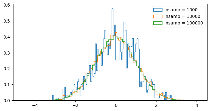
This module can also be used to plot discrete samples from a probability distribution.
# Draw samples from a Gaussian and plot them
mu = 0
sigma = 1
plt.figure()

#nsamp = 1000
for nsamp in [1e3,1e4,1e5]:
    samples = mu + sigma * np.random.randn(int(nsamp))
    plt.hist(samples, bins=100, histtype='step',lw=4,label='nsamp = {}'.format(int(nsamp)), density=True)
plt.legend();
In order to access data stored on the collective Google Drive, you must mount your drive to the notebook before accessing files. This requires authentication to allow Google Colab to access your files on your Google account.
from google.colab import drive
drive.mount('/content/drive')
Drive already mounted at /content/drive; to attempt to forcibly remount, call drive.mount("/content/drive", force_remount=True).
Once you have authenticated, you can access your own Drive in addition to any shared drives. We recommend adding a shortcut to the shared PHYSICS100_S2025 folder we have shared with you to your own drive by selecting More actions -> Organize -> Add Shortcut -> My Drive.
ls /content/drive/MyDrive/PHYSICS100_S2025/
data/ Lab0/ python_tutorial/
Let’s open a file similar to what will be output after a night of observing, FITS files. FITS files are composed of HDUs, or Header/Data Units. In almost all cases for this course, there will only be one HDU per file. The HDU contains a header, which gives information about the image, and the data, which is the image itself (although this does not always have to be the case, e.g. the light curve example below). For more information on the FITS file format, see this introduction.
In this tutorial, we will be looking at an image of the Whirlpool galaxy.
# Open the FITS file using the fits python module
filename = '/content/drive/MyDrive/PHYSICS100_S2025/python_tutorial/m51_2024_04_28-0001_B.fit'
whirlpool_hdu = fits.open(filename)
print(type(whirlpool_hdu))

# Grab the header and data
whirlpool_header = whirlpool_hdu[0].header
whirlpool_data = whirlpool_hdu[0].data

# print the header
whirlpool_header
<class 'astropy.io.fits.hdu.hdulist.HDUList'>
SIMPLE  =                    T
BITPIX  =                   16 /8 unsigned int, 16 & 32 int, -32 & -64 real
NAXIS   =                    2 /number of axes
NAXIS1  =                 2394 /fastest changing axis
NAXIS2  =                 1597 /next to fastest changing axis
BSCALE  =   1.0000000000000000 /physical = BZERO + BSCALE*array_value
BZERO   =   32768.000000000000 /physical = BZERO + BSCALE*array_value
DATE-OBS= '2024-04-29T04:04:46.50' /YYYY-MM-DDThh:mm:ss observation, UT
EXPTIME =   30.000000000000000 /Exposure time in seconds
EXPOSURE=   30.000000000000000 /Exposure time in seconds
SET-TEMP=  -15.000000000000000 /CCD temperature setpoint in C
CCD-TEMP=  -15.100000000000000 /CCD temperature at start of exposure in C
XPIXSZ  =   15.039999999999999 /Pixel Width in microns (after binning)
YPIXSZ  =   15.039999999999999 /Pixel Height in microns (after binning)
XBINNING=                    4 /Binning factor in width
YBINNING=                    4 /Binning factor in height
XORGSUBF=                    0 /Subframe X position in binned pixels
YORGSUBF=                    0 /Subframe Y position in binned pixels
READOUTM= 'Mode0   ' /          Readout mode of image
FILTER  = 'B       ' /          Filter used when taking image
IMAGETYP= 'Light Frame' /       Type of image
FOCALLEN=   0.0000000000000000 /Focal length of telescope in mm
APTDIA  =   0.0000000000000000 /Aperture diameter of telescope in mm
APTAREA =   0.0000000000000000 /Aperture area of telescope in mm^2
EGAIN   =  0.24665763974189758 /Electronic gain in e-/ADU
SBSTDVER= 'SBFITSEXT Version 1.0' /Version of SBFITSEXT standard in effect
GAIN    =                  100
OFFSET  =                   50
SWCREATE= 'MaxIm DL Version 6.40 240906 119MY' /Name of software
SWSERIAL= '119MY-HA61R-3FJ4C-458S4-1Y82K-U8' /Software serial number
FOCUSSSZ=   10.000000000000000 /Focuser step size in microns
JD      =   2460429.6699826387 /Julian Date at time of exposure
JD-HELIO=   2460429.6656362992 /Heliocentric Julian Date at time of exposure
OBJECT  = 'm51_2024_04_28'
TELESCOP= '        ' /          telescope used to acquire this image
INSTRUME= 'ASI Camera (2)'
OBSERVER= '        '
NOTES   = '        '
ROWORDER= 'TOP-DOWN' /          Image write order, BOTTOM-UP or TOP-DOWN
FLIPSTAT= 'Mirror  '
SWOWNER = 'Dr. Keith Thompson' /Licensed owner of software
CTYPE1  = 'RA---TAN'           / first parameter RA,    projection TANgential
CTYPE2  = 'DEC--TAN'           / second parameter DEC,  projection TANgential
CUNIT1  = 'deg     '           / Unit of coordinates
EQUINOX =               2000.0 / Equinox of coordinates
CRPIX1  =  1.197500000000E+003 / X of reference pixel
CRPIX2  =  7.990000000000E+002 / Y of reference pixel
CRVAL1  =  2.024936480229E+002 / RA of reference pixel (deg)
CRVAL2  =  4.719107556636E+001 / DEC of reference pixel (deg)
CDELT1  =  1.886027378426E-004 / X pixel size (deg)
CDELT2  =  1.890169267863E-004 / Y pixel size (deg)
CROTA1  = -1.080209939324E+002 / Image twist X axis (deg)
CROTA2  = -1.080784868706E+002 / Image twist Y axis (deg) E of N if not flipped.
CD1_1   = -5.834717149125E-005 / CD matrix to convert (x,y) to (Ra, Dec)
CD1_2   =  1.793504956801E-004 / CD matrix to convert (x,y) to (Ra, Dec)
CD2_1   = -1.796855988431E-004 / CD matrix to convert (x,y) to (Ra, Dec)
CD2_2   = -5.865564065045E-005 / CD matrix to convert (x,y) to (Ra, Dec)
PLTSOLVD=                    T / Astrometric solved by ASTAP v2024.03.21.
COMMENT 7  Solved in 0.1 sec. Offset 3.8".
WARNING = 'Warning inexact scale! Set FOV=0.30d or scale=0.7"/pix or FL=4559mm '
Note that the above object is an HDUList, and although it only has one element we still need to index by 0 to grab the header and data. More information on handling objects with this module can be found here. There’s a lot of information contained in the header about both the image and the telescope, and later labs will go through what is most important for image processing.
If you know what variable you want from the header, you can index the header object with a string.
filter = whirlpool_header['FILTER']
print(f'This image was taken with the {filter} filter')
This image was taken with the B filter
In the cell below: find and print the date of observation and exposure time for the image loaded above.
# TODO: above instructions
In addition to the header, the image can also be plotted (again using matplotlib).
plt.imshow(whirlpool_data, vmin=np.median(whirlpool_data)-2*np.std(whirlpool_data),vmax=np.median(whirlpool_data)+5*np.std(whirlpool_data))
<matplotlib.image.AxesImage at 0x7e5fe83fa250>
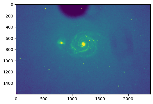
The vmin and vmax parameters above define the data range that the image covers. Try plotting the image without defining vmin and vmax, and describe what changes. Do you have any guesses why this change would occur?
# TODO: above instructions
FITS files don’t only contain astronomical images! Let’s take a look at a light curve.
# plot curve from a data file
# kepler light curve
datadir = '/content/drive/MyDrive/PHYSICS100_S2025/'
datadir += 'python_tutorial/python_tutorial_FITS/'
infiles = glob.glob(datadir + '*.fits')
print(len(infiles))
print(infiles[0])
15
/content/drive/MyDrive/PHYSICS100_S2025/python_tutorial/python_tutorial_FITS/kplr011904151-2009131105131_llc.fits
We can use the fits functionality to open the data file, index the second extension ([1]) and access the various attributes of the data, then plot it (with labels!):
kepler_hdulist = fits.open(infiles[0])
print(type(kepler_hdulist))
data = kepler_hdulist[1].data
x = data['TIME']
y = data['SAP_FLUX'] # Simple Aperture Flux
yerr = data['SAP_FLUX_ERR']

plt.errorbar(x,y,yerr=yerr)
plt.xlabel('Time (s)')
plt.ylabel('Flux (cts)')
<class 'astropy.io.fits.hdu.hdulist.HDUList'>
Text(0, 0.5, 'Flux (cts)')
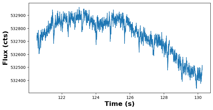
Note that above the HDUList object does contain more than one element, and the data we are looking for is in the second index.
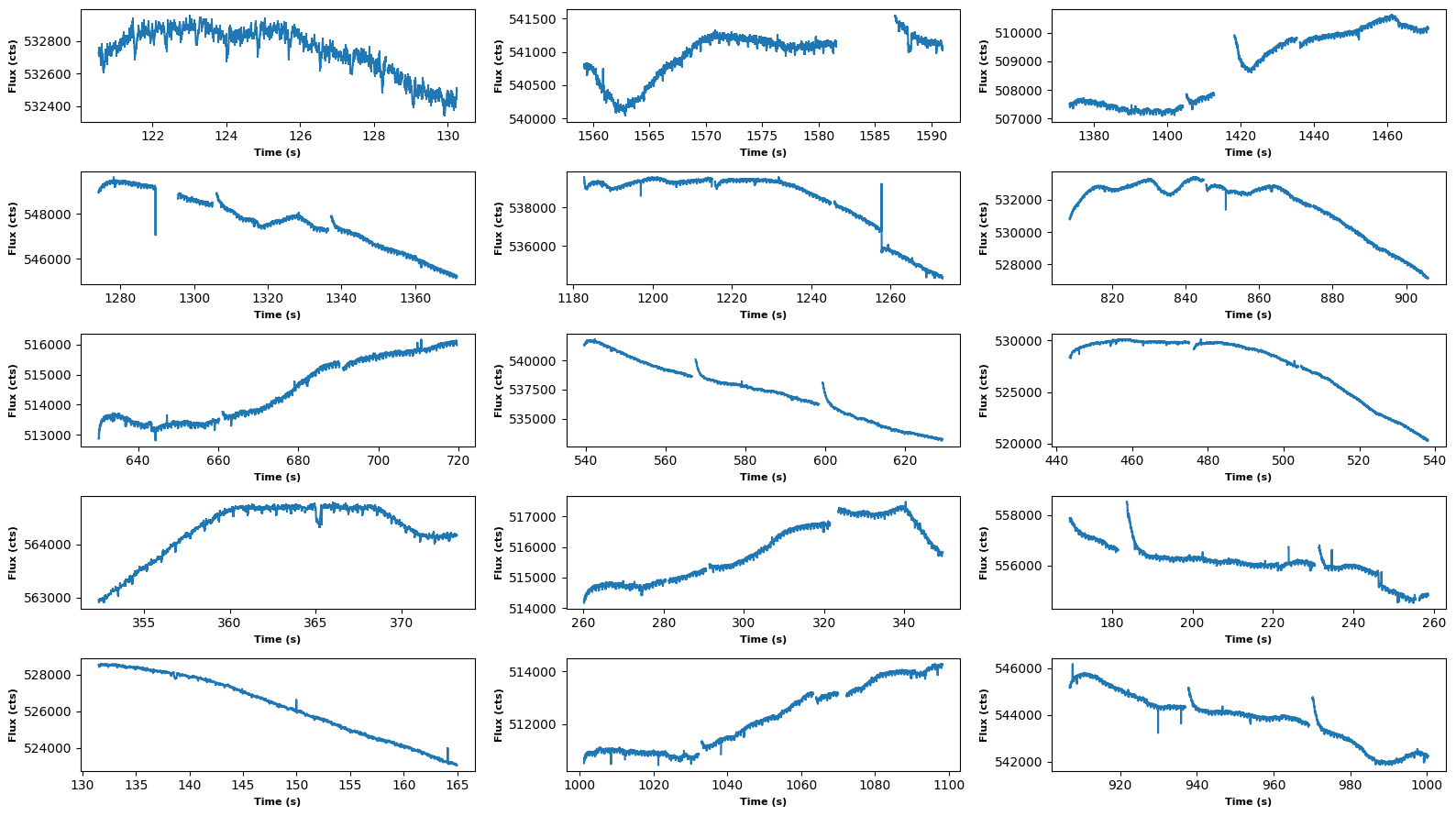
fig, axarr = plt.subplots(5, 3, figsize=(16.,9.))
for i, infile in enumerate(infiles):
    data = fits.open(infile)[1].data
    x = data['TIME']
    y = data['SAP_FLUX'] # Simple Aperture Flux
    yerr = data['SAP_FLUX_ERR']

    axarr[i // 3, i % 3].errorbar(x,y,yerr=yerr)
    axarr[i // 3, i % 3].set_xlabel('Time (s)',size=8)
    axarr[i // 3, i % 3].set_ylabel('Flux (cts)',size=8)

plt.tight_layout()
If you have any more questions with FITS files, please let us know!