Notes: Review of Probability

Containing:

• a review of the most relevant tools of mathematical probability
• some common probability distributions to be familiar with

Terminology and axioms

We'll keep things general at the start. Consider the set of all possible answers/outcomes for a given question/experiment. This is called the sample space, $\Omega$. A subset of $\Omega$ is called an event, $E$.

The probability of an event, $P(E)$, is a real function satisfying certain requirements known as the axioms of probability:

Axioms of probability

• $\forall E: 0 \leq P(E) \leq 1$
• $P(\Omega) = P\left(\bigcup_{\mathrm{all~}i} E_i\right) = 1$
• If $E_i$ are mutually exclusive, $P\left(\bigcup_i E_i\right) = \sum_i P(E_i)$

This dry definition provides a function with the right properties to describe our intuitive understanding of probability. In particular, if some experiment can in principle be repeated many times, independently and under identical conditions, then the fraction of outcomes $E$ will tend to $P(E)$. Probabilities can also be applied in circumstances that do not lend themselves to numerous, independent and identical repetition (that is, to circumstances that might actually exist in reality). In this case, the probability can be interpreted as a weight associated with evidence, information, knowledge, or belief. Although the word "subjective" is often used in this context, this doesn't imply a lack or rigor. The theory is still fully mathematical, and as such people should agree on the outcome of calculations based on the same starting assumptions, whatever their opinions might be. (They can disagree about the starting assumptions, but that's a different story.)

For those who have studied statistical mechanics, even if you haven't formally studied probability, the language above may seem familiar. In particular, you might have seen this when studying the microcanonical ensemble - if $\Omega$ is the set of states available to a system of fixed energy, the fundamental assumption of statistical mechanics is that all of those states are equally probable to occur.

Random variables and their distributions

Any quantity whose value can only be described probabilistically (i.e. that is not known with certainty) is called random. To be clear, "random" does not mean that nothing is known about the value of the variable; the form of its probability distribution may, in fact, be known precisely. This is analogous to the idea that it's possible to know the precise state of a quantum system, and make precise predictions about the frequency of different measurement outcomes, without knowing with certainty what the outcome of a specific measurement will be.

Very often, the events we're concerned with correspond to the different values that a random variable might have, with the sample space corresponding to the real numbers, non-negative real numbers, non-negative integers, etc., depending on the variable in question.

The axioms translate to this case straightforwardly, e.g. for an integer-valued variable $n$, the second axiom, $P(\Omega)=1$, becomes the normalization condition

$\sum_{n'=-\infty}^{\infty} P(n=n') = 1$.

For discrete random variables, like $n$ in this example, $P(n=n')$ is a function of $n'$ and is a probability. This is sometimes called the probability mass function (PMF) of $n$.

The corresponding function for a continuous random variable (e.g. a real number) is the probability density function (PDF), e.g. $p(x=x')$ for a real-valued $x$. However, it's important to realize that a PDF is not a probability! $p(x=x')$ is also not, in general, dimensionless (its dimensions are the inverse of $x$'s). However, any integrals of a PDF are probabilities, for example

• $p(x=x') \, dx'$
• $P(x_0 < x < x_1) = \int_{x_0}^{x_1} dx' \, p(x=x')$

are both probabilities.

As the notation $p(x=x')$ rapidly becomes cumbersome, we will be lazy and simply write $p(x)$ from now on. This should be interpreted as a function of $x$, the value of a random variable whose identity should normally be clear from the choice of symbol.

The distinction between probability mass and density is highly relevant if we ever want to change variables, e.g. $x\rightarrow y(x)$. In particular, $p(y) \neq p[x(y)]$. Instead, it turns out,

$p(y) = p(x) \left|\frac{dx}{dy}\right|$.

Things are more straightforward for probability mass: $P(y=Y)$ is the sum of $P(x)$ for all the values of $x$ that give $y(x)=Y$. To keep this distinction straight, we will use capital $P$ for probability, and lower-case $p$ for probability density.

Pointing back to the last section, a PMF tells us how likely a variable is to have any given value. A PDF tells us the relative probability of different values, and can be integrated to tell us the absolute probability in some range. In the limit (?) where we can do infinitely many realizations of equivalent random variables, these functions correspond to the fraction of realizations that would be observed with each value. However, it's important to accept that, while any reasonable definition of probability will include this hypothetical long-run frequency behavior as a consequence, it must also be well defined in the absence of infinitely many independent trials to be useful. This is obvious in the case of, say, cosmology (good luck producing any additional realizations of the Universe, let alone many of them), but no matter what type of experiment we're engaged in, we will ultimately need to reason about probabilities corresponding to the outcome of that non-infinitely-repeated experiment.

More probabilistic functions

The cumulative distribution function (CDF) is the probability that $x\leq x'$ as a function of $x'$. It's sometimes referred to simply as the "distribution function". This is obviously unnecessarily confusing, so we will not do so.

The CDF is usually written

$F(x') = P(x \leq x') = \int_{-\infty}^{x'} p(x=s)ds$.

It is, necessarily, non-decreasing and bounded by zero and one. For distributions over a continuous variable, the derivative of the CDF is the PDF.

The quantile function is the inverse of the CDF, $F^{-1}(\mathcal{P})$. It's argument is a probability, and it returns a quantile which lives in the same space as $x$. For example, the median of a distribution is $F^{-1}(0.5)$. A quantile is conceptually the the same as a percentile, except that one is a function of probability (between 0 and 1), while the other is a function of percentage probability (between 0 and 100).

Simple example: an unfair coin toss

We flip a coin which is weighted to land on heads a fraction $q$ of the time. To make things numeric, let $X=0$ for stand for an outcome of tails and $X=1$ for heads. We have the discrete PMF

• $P(0) = 1-q$,
• $P(1) = q$;

and the corresponding CDF

• $F(0) = 1-q$,
• $F(1) = 1$.

The quantile function would be

• $F^{-1}(\mathcal{P})$ undefined for $\mathcal{P}<1-q$,
• $F^{-1}(\mathcal{P}) = 0$ for $1-q \le \mathcal{P} < 1$,
• $F^{-1}(\mathcal{P}=1) = 1$.

Multivariate probability distributions

Things get more interesting when we deal with joint distributions of multiple events, $p(X=x$ and $Y=y)$, or just $p(x,y)$. We might visualize such a function using contours of equal probability, for example:

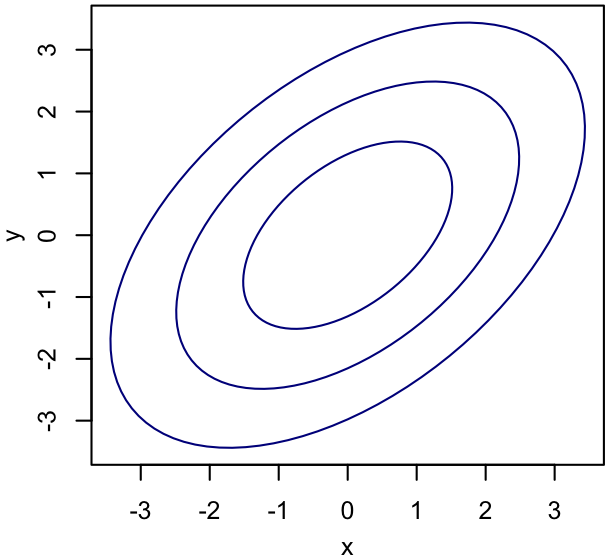For the uninitiated, these iso-probability contours qualitatively tell us the following:

• The peak probability density is somewhere in the center of the figure (the contours aren't labeled, but it's fair to assume the smaller ones are higher probability, since the integral of $p(x,y)$ must be normalized).
• Moving away from the peak along the longer axis of the ellipse-like contours, the probability density falls off more slowly than along the shorter axis.

We often refer to elongated shapes like this one as revealing degeneracies between parameters. The meaning here is (approximately) similar to the use of "degenerate" in quantum mechanics: something - here the probability density rather than the energy of a system - is (approximately) conserved along a particular locus in parameter space. For good measure, we might also refer to the two parameters as correlated, with essentially the same meaning.

There are various meaningful manipulations and reductions of multivariate distributions to know.

The marginal probability of $y$, $p(y)$, means the probability of $y$ irrespective of what $x$ is. Mathematically, this corresponds to summing $p(x,y)$ over all possible values of $x$, for a given $y$:

$p(y) = \int dx \, p(x,y)$.

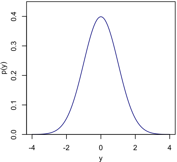You can see that the result is a function of $y$ only, and that information about the structure of the 2-dimensional function $p(x,y)$ is gone.

The conditional probability of $y$ given a value of $x$, $p(y|x)$, is most easily understood this way:

$p(x,y) = p(y|x)\,p(x)$.

That is, the probability of getting $x$ AND $y$ can be factorized into the product of probabilities of

• getting $x$ regardless of $y$, and at the same time
• getting $y$ given $x$.

$p(y|x)$ is a normalized slice through $p(x,y)$ rather than an integral. Specifically, $1/p(x)$ is exactly the coefficient needed to normalize things such that, integrating the identity above, $\int dy \, p(y|x) = \int dy \, p(x,y)/p(x) = 1$.

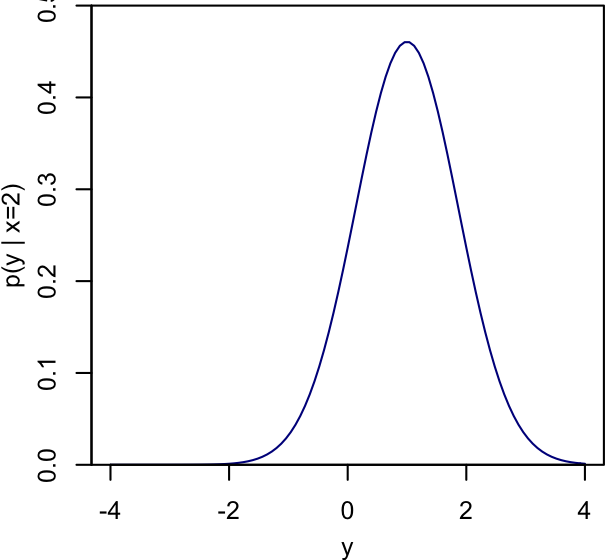In this example, comparing to the 2-dimensional plot above, you can see that the peak of $p(y|x)$ will move depending on what value of $x$ is conditioned on.

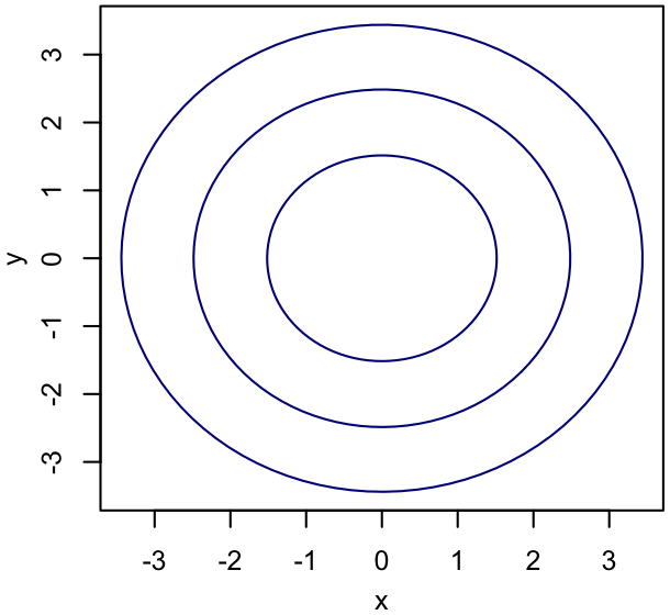
In the special case where $p(y|x) = p(y)$, $x$ and $y$ are independent. Equivalently, $p(x,y) = p(x)\,p(y)$. It should be clear that this requires the isoprobability contours to look qualitatively different than in the example above - in particular, the mean of $p(y|x)$ has better not depend on $x$, so the "axes" of the iso-probability contours must be aligned with the $x$ and $y$ axes (the contours need not be circular, though). In this case, we could refer to the two parameters as uncorrelated and/or not degenerate.

For completeness, one can also define the straightforward generalization of the CDF,

$F(x',y') = P(x \leq x', y \leq y')$.

However the inverse (quantile) function is now multivalued, which can make them less useful, at least for some purposes. We probably won't see either the CDF or quantile function used in the multivariate case.

Probability calculus

The section above outlines the basic operations we can perform on probabilities and probability densities, namely marginalization and conditioning. Rather than diving into the formalities of probability as a branch of mathematics, we hope that learning by example in the later notes will be enough. Still, here are a couple of basic rules that will hopefully avoid confusion:

1. One cannot marginalize over a variable if it appears only to the right of a "|", because variables that are conditioned on are necessarily fixed as far as the expression they appear in is concerned.
2. Pedantically applying the definition of conditional probability and substituting into an equation is much safer than trying to intuit when and where "|" can just be dropped in.

Those who are dying to read a more comprehensive yet not terribly accessible reference (which quickly gets far ahead of what we need for the moment), are invited to start here.

The most convenient mathematical shortcuts ever

Let us reiterate that probability densities must obey the various rules and definitions above. These are not properties that you need to prove when using them.

To put it differently, probability densities are extremely easy functions to work with, compared with what one normally sees in graduate physics. We will technically be performing very difficult differential equations and integrals, but will mostly be doing so numerically. This is because the properties of PDFs tend to simplify those calculations that can be done on paper to algebraic manipulation rather than calculus. Some examples:

• The indefinite integral of a PDF never has to be carried out. Ever. It's 1. Move on.
• Let's say you have a PDF on the left hand side of an equation, and a jumble on the right hand side. If you can recognize the functional dependence of the RHS as belonging to a known (i.e. named) distribution, and thereby identify the values of its parameters, you are done. There is no need to simplify the jumble by brute force, because the fact that the RHS is a PDF, combined with normalization condition, means it is necessarily equal to the PDF of the distribution you recognized, with nothing left over.
• Say we're handed a jumble representing a multivariate PDF over $x$ and $y$. If it facorizes into a term that depends on $x$ only and a term that depends on $y$ only, then we can immediately say that $x$ and $y$ are independent, and what the functional forms of their marginal PDFs are. If those PDFs are known distributions, we can immediately write down $p(x)$ and $p(y)$. We again don't need to actually manipulate the constants to show that this will work, because normalization requires it.
• Similarly, if we can factor such a multivariate distribution into a known PDF that depends on $x$ only, and another that depends on both $x$ and $y$, we can immediately identify $p(x)$ and $p(y|x)$ without suffering through explicit simplification.

Exercise

Here is a quick test of your understanding of some of the concepts so far. (Solutions are at the end of the notes.)

Take the coin tossing example from earlier, where $P(\mathrm{heads})=q$ and $P(\mathrm{tails})=1-q$ for a given toss. Assume that this holds independently for each toss, and that the coin is tossed twice.

Find:

1. The conditional probability that both tosses are heads, given that the first toss is heads.
2. The conditional probability that both tosses are heads, given that at least one of the tosses is heads.
3. The marginal probability that the second toss is heads.

Writing out the probability of all 4 possible outcomes of the 2 coin tosses and then reasoning about them is a completely legitimate approach here, and even preferable to relying on formulae. But it's still a good idea to see those formulae in action, producing the same result.

For more practice manipulating probabilities see the essential probability tutorial.

Some standard probability distributions

For reference, here is a non-exhaustive list of distributions that commonly arise. They are "standard" in the sense that they have been studied since the days of pencil and paper derivations, so lots of analytic properties are known. Various functions are also usually implemented for you in software (e.g. scipy.stats). This is not remotely a comprehensive list, and Wikipedia is a good first stop if you run into something unfamiliar, or suspect the function you're looking at must be a standard PDF but don't know its name.

Bernoulli distribution

This is the example used above. It's support (the space over which the PDF or PMF is defined) is a discrete set of cardinality 2 (i.e. heads or tails, true or false, 1 or 0), and the distribution's only parameter is the probability of "success" (usually defined as heads/true/1), $q$.

Not especially useful on its own, apart from as an introductory example. But, if we have $N$ independent Bernoulli trials, the total number of successes follows the...

Binomial distribution

... whose PMF is $P(k|q,n) = {n \choose k} q^k (1-q)^{n-k}$ for $k$ successes. ${n \choose k}$ is the combinatoric "choose" function, $\frac{n!}{k!(n-k)!}$.

The Binomial distribution is additive, in that the sum of two Binomial random variables with the same $q$, respectively with $n_1$ and $n_2$ trials, also follows the Binomial distribution, with parameters $q$ and $n_1+n_2$.

This distribution might be useful for inferring the fraction of objects belonging to one of two classes ($q$), based on typing of an unbiased but finite number of them ($n$). (The multinomial generalization would work for more than two classes.)

Or, consider the case that each Bernoulli trial is whether a photon hits our detector in a given, tiny time interval. For an integration whose total length is much longer than any such time interval we could plausibly distinguish, we might take the limit where $n$ becomes huge, thus reaching the...

Poisson distribution

... which describes the number of successes when the number of trials is in principle infinite, and $q$ is correspondingly vanishingly small. It has a single parameter, $\mu$, which corresponds to the product $qn$ when interpreted as a limit of the Binomial distribution. The PMF is

$P(k|\mu) = \frac{\mu^k e^{-\mu}}{k!}$.

Like the Binomial distribution, the Poisson distribution is additive. It has the following (probably familiar) properties:

• Expectation value (mean) $\langle k\rangle = \mu$,
• Variance $\left\langle \left(k-\langle k \rangle\right)^2 \right\rangle = \mu$.

For Sufficiently Large values of $\mu$, the Poisson distribution is well approximated by the...

Normal or Gaussian distribution

... which is, more generally, defined over the real line as

$p(x|\mu, \sigma) = \frac{1}{\sqrt{2\pi\sigma^2}} \exp \left[ -\frac{(x-\mu)^2}{2\sigma^2} \right]$,

and has mean $\mu$ and variance $\sigma^2$. With $\mu=0$ and $\sigma=1$, this is known as the standard normal distribution.

Because Gauss was a physicist and astronomer (presumably), you can expect to see "Gaussian" more often in the (astro)physics literature. Statisticians normally say "normal". (According to the Wikipedia, Gauss actually coined the terminology "normal distribution", meant in the sense of "orthogonal".)

The limiting relationship between the Poisson and Normal distributions is one example of the central limit theorem, which says that, under quite general conditions, the average of a large number of random variables tends towards normal, even if the individual variables are not normally distributed or not fully independent. Whether and how well it applies, and just what "large number" means in any given situation, is a practical question more than anything else, at least in this course. Lots of math has been expended proving inequalities that hold under some assumptions or others, but in general the only way to know is to compare the approximate normal distribution with the unapproximated distribution in question (by simulation).

The bottom line is that the Gaussian distribution shows up quite often, and is "normally" a reasonable guess in those situations where we have to make a choice and have no better ideas. Historically, it was also an incredibly useful approximation due to its mathematical simplicity; these days we can often get more out of the data by not making such approximations, except as a last resort. On that note, be aware that intentionally binning up data, when doing so throws out potentially useful information (e.g. combining Poisson measurements made at different times if we are trying to measure the lightcurve of some source), in the hopes of satisfying the central limit theorem is generally frowned upon in this class.

Finally, the sum of squares of $\nu$ standard normal variables follows the...

Chi-square (or chi-squared, or $\chi^2$) distribution

... whose PDF is

$p(x|\nu) = \frac{x^{\nu/2-1} e^{-x/2}}{2^{\nu/2}\Gamma(\nu/2)}$,

where $\Gamma$ is the gamma function and $\nu$ is a positive integer. This distribution is also sometimes abbreviated as $\chi^2_\nu$, explicitly showing the parameter, $\nu$.

Notation

When a probability distribution is known to be one of these standard distributions, we will often use its name explicitly. So,

$\mathrm{Normal}(x|\mu,\sigma)$

should be read as a Gaussian PDF over $x$ with parameters $\mu$ and $\sigma$, like a more specific version of $p(x|\mu, \sigma)$. The notation

$\mathrm{Normal}(\mu,\sigma)$

would refer to the distribution generally (i.e. not specifically to its density function), as in "$x$ is distributed as $\mathrm{Normal}(\mu,\sigma)$".

Exercise solutions

1. $P(X=1,Y=1|X=1) = P(X=1,Y=1)/P(X=1) = q^2/q = q$

2. $P(X=1,Y=1|X=1\cup Y=1) = P(X=1,Y=1)/P(X=1\cup Y=1)$

$\quad = P(X=1,Y=1)/[P(X=1,Y=1)+P(X=1,Y=0)+P(X=0,Y=1)]$

$\quad = q^2/[q^2 + 2q(1-q)]$

3. $P(Y=1) = P(X=0,Y=1) + P(X=1,Y=1) = q(1-q) + q^2 = q$