Physics89L
Notes and materials for Week 6
Topics covered: Least-squares fitting with a function minimizer.
- Course material
Data analysis topics
This week we are going to be how to perform least-squares fitting with a function minimizer.
Least squares fitting
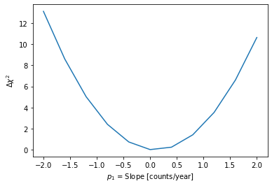
Last week we saw that we could estimate the model parameters that gave the best agreement to the data by scanning over the
parameters and computing the chi**2 for each value of the parameter.
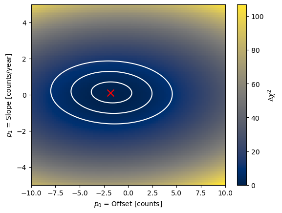
We also did this for two parameters at once. That gave us a plot that looks like this:
This week we are going to use an algorithm that finds the set of parameters that minimize the chi**2 and give the best fit.
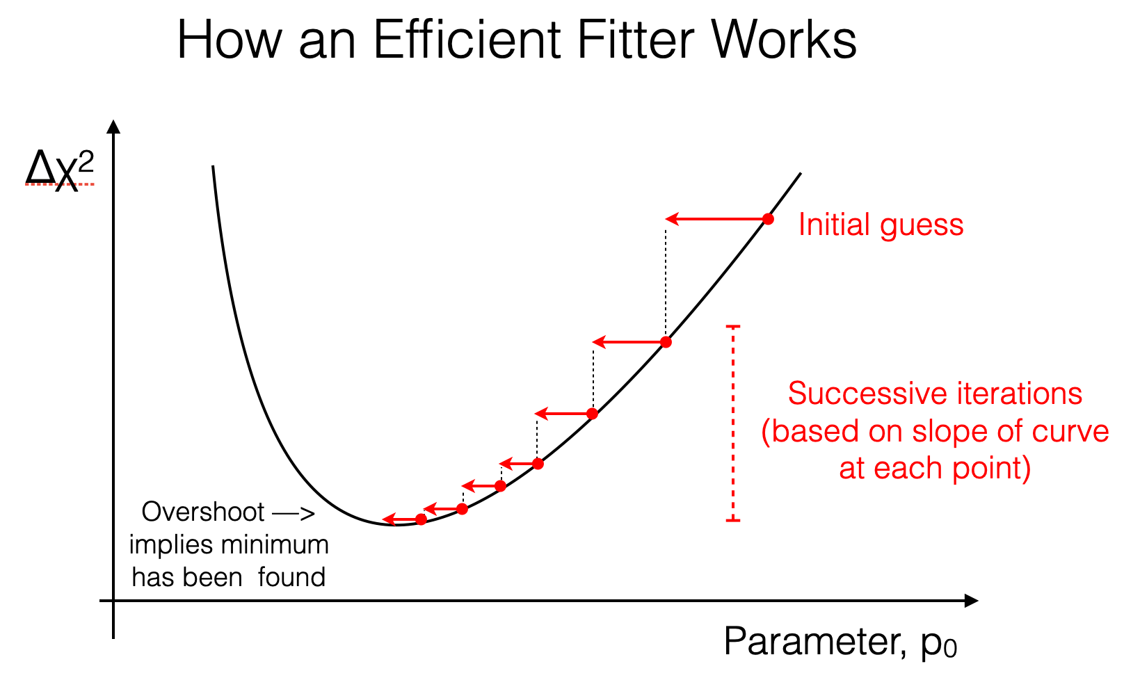
There are a number of different algorithms that can find the parameters that minimize the chi**2. What they have in common is that
they start out with an initial guess, and then try to improve on that guess until they believe that they are very close to the best
solution.
One of the most basic algorithms is the Nelder-Mead algorithm, which calculates the function values at different points of a “simplex”. A simplex in 2D space is just a triangle. The algorithm is initialized with three points, which define the triangle. For each step of the algorithm, the function values at the triangle vertices are calculated. The algorithm then evaluates nearby points, and then the point with the largest value of the function is then updated with a nearby point to define a new triangle. This is repeated until the criteria for “convergence” is reached.
Other minimization algorithms also make use of the first and second derivatives of the function with respect to the parameters. This gives you information about the shape of the function and which direction to “step” to find a minimum. These are often referred to as gradient-descent and Newton methods. The details of how these algorithm work are well beyond the scope of this class, but this is a very useful tool to be familiar with.
Scientific context and resources
In the second Jupyter notebook we will be using the output of some data analysis done using the spectrum of a distant object as measured by the Sloan Digital Sky Survey.
Over the course of 20 years, SDSS observed 35% of the sky and cataloged about 1 billion stars and galaxies.
It addition to taking images of such a large part of the sky, SDSS also measured the spectrum of the light from over 4 million objects.
The spectra show the energy flux (i.e., the amount of energy per area, per time) as a function of wavelength for two objects.
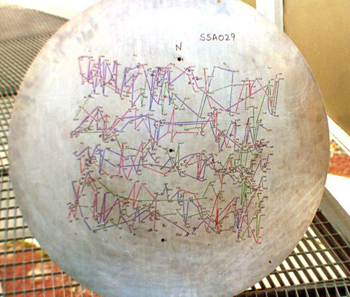
The spectra are obtained by feeding an individual optical fibre for each target through a hole drilled in an aluminum plate. The light from the fiber is then passed into a diffraction grating to separate out the different wavelength so that the spectrum for that target can be measured. The diffracted light was the directed to an array of sensors, so that each sensor measured the amount of light at a different wavelength.
Each hole is positioned specifically for a selected target, so every field in which spectra are to be acquired requires a unique plate. In spectroscopic mode, the telescope tracks the sky in the standard way, keeping the objects focused on their corresponding fibre tips.
Here is a picture of one such aluminum plate:
Here are a couple of spectra:
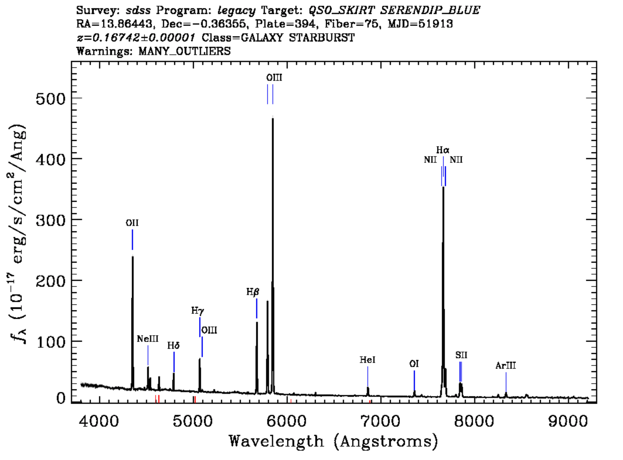
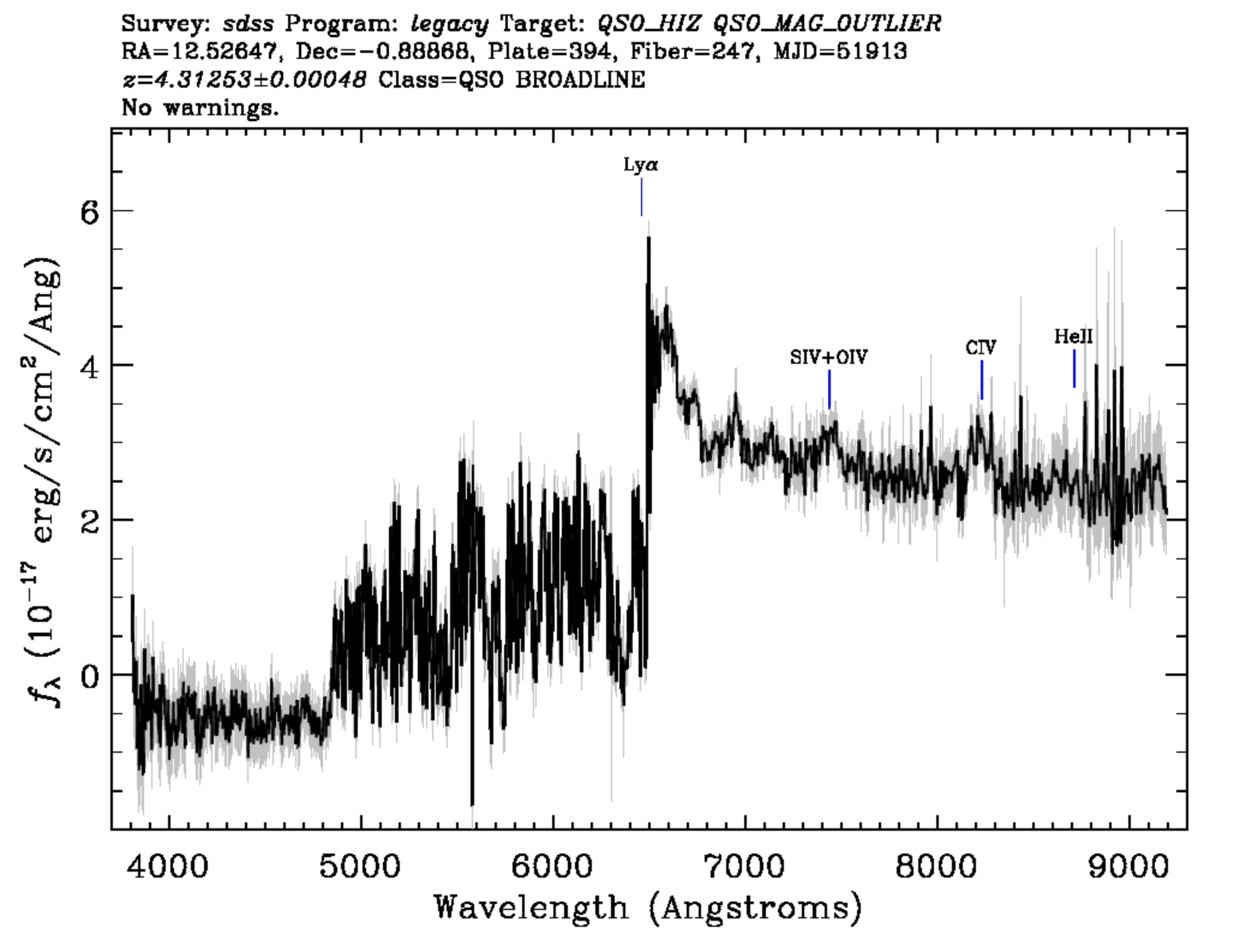
The figures have been helpfully annotated, showing the lines that correspond to particular atomic transitions. By comparing the measured wavelength of the lines with the know emission wavelength we can measure the Dopper shift for each object.
Python functions reference
We will not be using a lot of new python functions this week. Here are the important ones that we will be using.
| Function Name | What it does |
|---|---|
| scipy.optimize.minimize | Find the set of parameters that minimize a cost function |